SciPy - interpolate.KroghInterpolator() Function

scipy.interpolate.KroghInterpolator() is a function in the scipy.interpolate module for polynomial interpolation using the Krogh or Hermite method. It constructs an interpolating polynomial that passes through a given set of data points which may include derivatives at these points.

This allows for both interpolation of function values and derivative values by providing a flexible way to model smooth curves through data with specified slopes. The interpolator is useful for high-accuracy interpolation especially when derivatives are known and can handle situations where the x-values contain repeated points.

Syntax

Following is the syntax of the function scipy.interpolate.KroghInterpolator() to perform polynomial interpolation −

scipy.interpolate.KroghInterpolator(xi, yi, axis=0)

Parameters

Here are the parameters of the scipy.interpolate.KroghInterpolator() function −

• xi(array-like): 1-D array of independent data points where interpolation is performed (x-values).
• yi(array-like, optional): Array of dependent data points (y-values). This can be multi-dimensional and in this case the axis specifies which axis of yi is the one corresponding to the dependent variable.
• axis(int, optional): Specifies the axis of yi along which to interpolate. By default axis=0 which means the interpolation is performed along the first axis (rows). If yi is multi-dimensional then this parameter allows us to apply interpolation along different axes.

Return Value

The scipy.interpolate.KroghInterpolator() function does not directly return a result when instantiated. Instead it returns an interpolator object which can be called like a function to evaluate the interpolating polynomial at different points.

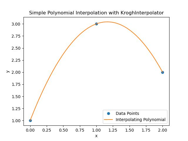
Simple Polynomial Interpolation

Following is a simple example of polynomial interpolation using scipy.interpolate.KroghInterpolator() function. In this example we have a set of data points and we want to construct a polynomial that passes through all of them −

from scipy.interpolate import KroghInterpolator
import numpy as np
import matplotlib.pyplot as plt

# Define data points
xi = np.array([0, 1, 2])
yi = np.array([1, 3, 2])

# Create the KroghInterpolator object
interpolator = KroghInterpolator(xi, yi)

# Use the interpolator to evaluate at new points
x_new = np.linspace(0, 2, 100)  # Generate 100 points between 0 and 2
y_new = interpolator(x_new)

# Plot original points and the interpolated polynomial
plt.plot(xi, yi, 'o', label='Data Points')  # Mark original points
plt.plot(x_new, y_new, label='Interpolating Polynomial')  # Interpolated polynomial curve
plt.legend()
plt.xlabel('x')
plt.ylabel('y')
plt.title('Simple Polynomial Interpolation with KroghInterpolator')
plt.show()

Here is the output of the scipy.interpolate.KroghInterpolator() function −

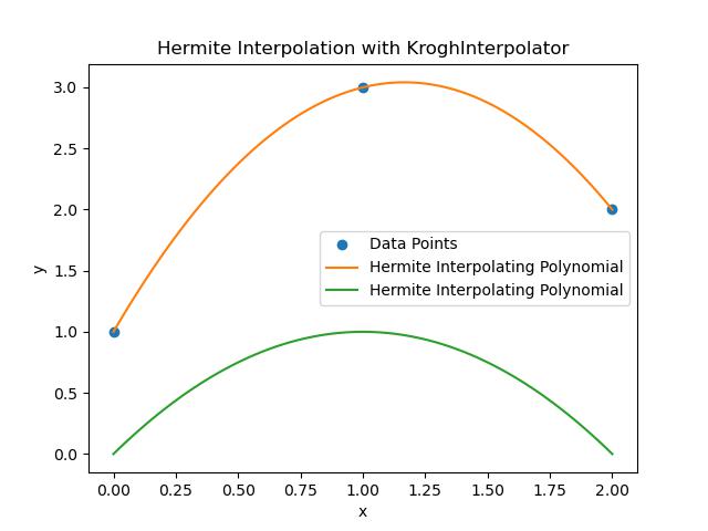
Hermite Interpolation with Derivatives

Hermite interpolation is a type of interpolation where both function values and derivatives are specified at each point. The KroghInterpolator() function in scipy.interpolate can handle this by allowing us to pass both the values and derivatives for each point. Below is the example of the Hermite Interpolation −

from scipy.interpolate import KroghInterpolator
import numpy as np
import matplotlib.pyplot as plt

# Define data points
xi = np.array([0, 1, 2])
yi = np.array([1, 3, 2])

# Create the KroghInterpolator object
interpolator = KroghInterpolator(xi, yi)

# Use the interpolator to evaluate at new points
x_new = np.linspace(0, 2, 100)  # Generate 100 points between 0 and 2
y_new = interpolator(x_new)

# Plot original points and the interpolated polynomial
plt.plot(xi, yi, 'o', label='Data Points')  # Mark original points
plt.plot(x_new, y_new, label='Interpolating Polynomial')  # Interpolated polynomial curve
plt.legend()
plt.xlabel('x')
plt.ylabel('y')
plt.title('Simple Polynomial Interpolation with KroghInterpolator')
plt.show()

Here is the output of the scipy.interpolate.KroghInterpolator() function used to perform Hermite Interpolation with Derivatives −

Interpolating Multiple Points

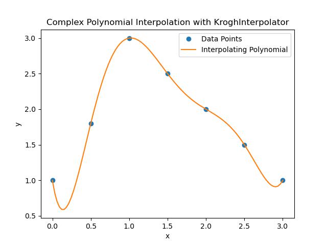
Here's an example of using KroghInterpolator to interpolate multiple data points. The idea is to pass a larger set of data points and have the interpolator construct a polynomial that smoothly passes through all of them −

from scipy.interpolate import KroghInterpolator
import numpy as np
import matplotlib.pyplot as plt

# Define more complex data points
xi = np.array([0, 0.5, 1, 1.5, 2, 2.5, 3])
yi = np.array([1, 1.8, 3, 2.5, 2, 1.5, 1])

# Create the interpolator object
interpolator = KroghInterpolator(xi, yi)

# Use the interpolator to evaluate at new points
x_new = np.linspace(0, 3, 100)
y_new = interpolator(x_new)

# Plot the original points and the interpolating polynomial
plt.plot(xi, yi, 'o', label='Data Points')  # Original points
plt.plot(x_new, y_new, label='Interpolating Polynomial')  # Interpolated curve
plt.legend()
plt.xlabel('x')
plt.ylabel('y')
plt.title('Complex Polynomial Interpolation with KroghInterpolator')
plt.show()

Here is the output of the scipy.interpolate.KroghInterpolator() function used to perform interpolation with multiple points −