SciPy - interpolate.RegularGridInterpolator() Function

scipy.interpolate.RegularGridInterpolator() is a function in SciPy designed for interpolating data on a regular grid in one or more dimensions. It creates an interpolation function based on values defined at grid points.

When users specify the grid coordinates and corresponding values and the interpolator then can compute values at any point within the grid using linear or nearest-neighbor interpolation methods.

It is efficient for multidimensional data and is particularly useful in applications such as numerical simulations where data is regularly spaced. This interpolator can also handle extrapolation beyond the grid boundaries by specifying a fill value.

Syntax

Following is the syntax of the function scipy.interpolate.RegularGridInterpolator() which is used to perform interpolation−

scipy.interpolate.RegularGridInterpolator(points, values, method='linear', bounds_error=True, fill_value=np.nan)

Parameters

Following are the parameters of the scipy.interpolate.RegularGridInterpolator() function −

• points: A sequence of 1D arrays defining the coordinates of the grid points in each dimension. The length of this sequence should be equal to the number of dimensions.
• values: An array of shape N_1, N_2, ..., N_d where N_i is the number of points along the i-th dimension. This array contains the values at the grid points defined by points.
• method: This is the interpolation method. The interpolation methods such as linear, nearest and we can also specify higher-order methods if desired.
• bounds_error: If True (default) then an error is raised when interpolation is requested for points outside the grid boundaries. If False then fill_value is used for out-of-bounds points.
• fill_value: Value to use for points outside the grid if bounds_error is False. The default value is np.nan.

Return Value

The scipy.interpolate.RegularGridInterpolator() function returns the interpolated values at the defined points.

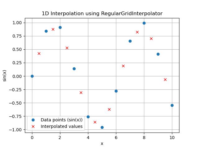
1D Interpolation

Following is the example of scipy.interpolate.RegularGridInterpolator() function in which well 1-d interpolate −

import numpy as np
from scipy.interpolate import RegularGridInterpolator
import matplotlib.pyplot as plt

# Define a 1D grid
x = np.linspace(0, 10, 11)  # x-coordinates (0, 1, 2, ..., 10)

# Define values on this grid (e.g., a function of x)
values = np.sin(x)  # Sample values (sine function)

# Create a RegularGridInterpolator object
interp_func = RegularGridInterpolator((x,), values)

# Points to interpolate at (these can be any value within the range of x)
xi = np.array([0.5, 1.5, 2.5, 3.5, 4.5, 5.5, 6.5, 7.5, 8.5, 9.5])

# Perform interpolation
interpolated_values = interp_func(xi)

# Print interpolated values
print("Interpolated values:", interpolated_values)

# Visualization
plt.plot(x, values, 'o', label='Data points (sin(x))')
plt.plot(xi, interpolated_values, 'x', label='Interpolated values', color='red')
plt.xlabel('x')
plt.ylabel('sin(x)')
plt.title('1D Interpolation using RegularGridInterpolator')
plt.legend()
plt.grid()
plt.show()

Here is the output of the scipy.interpolate.RegularGridInterpolator() function used for simple 1d interpolation −

Interpolated values: [ 0.42073549  0.87538421  0.52520872 -0.30784124 -0.85786338 -0.61916989
  0.18878555  0.82317242  0.70073837 -0.06595131]

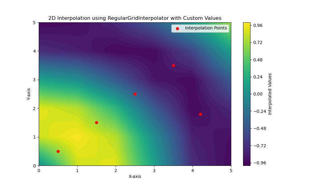
2D Interpolation with Custom Values

In this example we can perform 2D interpolation using scipy.interpolate.RegularGridInterpolator() with custom values in which we define a custom grid and use the interpolator to obtain values at arbitrary points −

import numpy as np
from scipy.interpolate import RegularGridInterpolator
import matplotlib.pyplot as plt

# Define 2D grid points
x = np.linspace(0, 5, 6)  # x-coordinates (0, 1, 2, 3, 4, 5)
y = np.linspace(0, 5, 6)  # y-coordinates (0, 1, 2, 3, 4, 5)

# Define custom values on the grid (a 2D function)
# For example, a simple function: z = f(x, y) = sin(sqrt(x^2 + y^2))
X, Y = np.meshgrid(x, y)  # Create a meshgrid for x and y
Z = np.sin(np.sqrt(X**2 + Y**2))  # Compute custom values

# Create the RegularGridInterpolator object
interp_func = RegularGridInterpolator((x, y), Z)

# Define points where we want to interpolate
xi = np.array([[1.5, 1.5], [2.5, 2.5], [3.5, 3.5], [4.2, 1.8], [0.5, 0.5]])

# Perform interpolation
interpolated_values = interp_func(xi)

# Print interpolated values
print("Interpolated values at specified points:", interpolated_values)

# Visualization
# Create a grid for visualization
xi_grid, yi_grid = np.meshgrid(np.linspace(0, 5, 50), np.linspace(0, 5, 50))
zi_grid = interp_func(np.array([xi_grid.ravel(), yi_grid.ravel()]).T).reshape(xi_grid.shape)

plt.figure(figsize=(10, 6))
plt.contourf(xi_grid, yi_grid, zi_grid, levels=50, cmap='viridis')
plt.colorbar(label='Interpolated Values')
plt.scatter(xi[:, 0], xi[:, 1], color='red', label='Interpolation Points', zorder=5)
plt.title('2D Interpolation using RegularGridInterpolator with Custom Values')
plt.xlabel('X-axis')
plt.ylabel('Y-axis')
plt.legend()
plt.show()

Here is the output of the scipy.interpolate.RegularGridInterpolator() function used for 2d interpolation −

Interpolated values at specified points: [ 0.71733399 -0.3696485  -0.84892675 -0.91681464  0.66767698]