SciPy - ndimage.black_tophat() Function

The scipy.ndimage.black_tophat() function in SciPy which is used to perform the black top-hat morphological filter on an input image. It subtracts the result of an erosion operation by using a structuring element from the original image by highlighting regions that are darker than their surroundings.

This filter is useful for detecting small, dark structures or spots. This function takes several parameters such as input (the image), size (defines the structuring element size), footprint (specifies the shape of the structuring element), mode (boundary handling) and origin (shifts the structuring element). The output is an image emphasizing dark regions relative to the surrounding area.

Syntax

Following is the syntax of the function scipy.ndimage.black_tophat() to implement Black Top-Hat Operation on an image −

scipy.ndimage.black_tophat(input, size=None, footprint=None, structure=None, output=None, mode='reflect', cval=0.0, origin=0)

Parameters

Following are the parameters of the scipy.ndimage.black_tophat() function −

• input: The input image or array which can be grayscale or binary, on which the black top-hat filter is applied.
• size(optional): This specifies the size of a square structuring element and overrides footprint and structure if provided.
• footprint(optional): A binary array defining the shape of the structuring element where non-zero elements determine the neighborhood.
• structure(optional): It is an array that explicitly specifies the structuring element. Overrides both size and footprint when provided.
• output(optional): This is an array where the result will be stored. If not provided, a new array is allocated.
• mode(optional): It determines how the filter handles image boundaries and this includes 'reflect', 'constant', 'nearest', 'mirror', and 'wrap'.
• cval(optional): The constant value to use when mode='constant' is selected. The default value is 0.0.
• origin(optional): This parameter controls the placement of the structuring element relative to the pixel being processed. The default value is 0.

Return Value

The scipy.ndimage.black_tophat() function returns with the same shape as the input array and highlights dark spots on a light background.

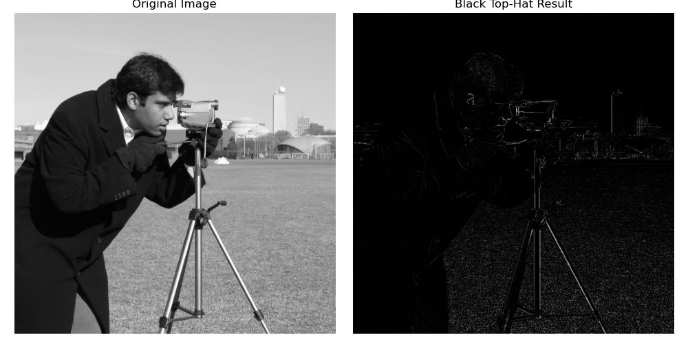
Basic Black Top-Hat Filtering (Default Values)

Following is an example which shows a simple Black Top-Hat filter applied to an image with a default square structuring element (3x3) with the help of scipy.ndimage.balck_tophat() function −

import numpy as np
import matplotlib.pyplot as plt
from scipy.ndimage import black_tophat
from skimage.data import camera

# Load the input image
image = camera()

# Apply Black Top-Hat filter with a default 3x3 structuring element
result = black_tophat(image, size=3)

# Display original and filtered images
plt.figure(figsize=(10, 5))
plt.subplot(1, 2, 1)
plt.title("Original Image")
plt.imshow(image, cmap='gray')
plt.axis('off')

plt.subplot(1, 2, 2)
plt.title("Black Top-Hat Result")
plt.imshow(result, cmap='gray')
plt.axis('off')

plt.tight_layout()
plt.show()

Here is the output of the function scipy.ndimage.black_tophat() which is used to implement basic Example of Black Top Hat −

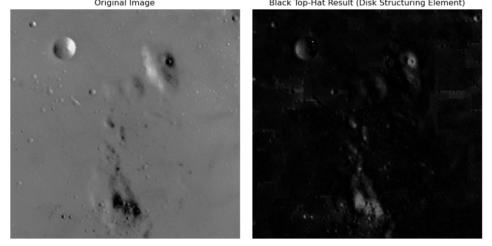
Using a Custom Structuring Element

In this example a custom disk-shaped structuring element is used for the Black Top-Hat filter −

import numpy as np
import matplotlib.pyplot as plt
from scipy.ndimage import black_tophat
from skimage.morphology import disk
from skimage.data import moon

# Load the input image
image = moon()

# Create a disk-shaped structuring element
structuring_element = disk(15)

# Apply Black Top-Hat filter using the custom structuring element
result = black_tophat(image, structure=structuring_element)

# Display original and filtered images
plt.figure(figsize=(10, 5))
plt.subplot(1, 2, 1)
plt.title("Original Image")
plt.imshow(image, cmap='gray')
plt.axis('off')

plt.subplot(1, 2, 2)
plt.title("Black Top-Hat Result (Disk Structuring Element)")
plt.imshow(result, cmap='gray')
plt.axis('off')

plt.tight_layout()
plt.show()

Here is the output of the function scipy.ndimage.black_tophat() which is used to implement custom disk Black Top Hat −

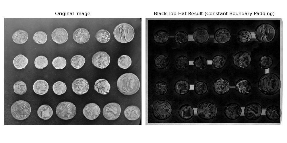
Boundary Handling with Constant Padding

Here is the example which shows how to handle image boundaries using constant padding when applying the Black Top-Hat filter −

import numpy as np
import matplotlib.pyplot as plt
from scipy.ndimage import black_tophat
from skimage.data import coins

# Load the input image
image = coins()

# Apply Black Top-Hat filter with constant padding at the boundaries
result = black_tophat(image, size=15, mode='constant', cval=0)

# Display original and filtered images
plt.figure(figsize=(10, 5))
plt.subplot(1, 2, 1)
plt.title("Original Image")
plt.imshow(image, cmap='gray')
plt.axis('off')

plt.subplot(1, 2, 2)
plt.title("Black Top-Hat Result (Constant Boundary Padding)")
plt.imshow(result, cmap='gray')
plt.axis('off')

plt.tight_layout()
plt.show()

Here is the output of the function scipy.ndimage.black_tophat() with constant boundary padding −