SciPy - ndimage.grey_erosion() Function

The scipy.ndimage.grey_erosion() is a function used to perform morphological erosion on grayscale images. Unlike the Binary erosion which operates on binary values (0 or 1) and grey erosion works with grayscale values. It replaces each pixel in the image with the minimum value within a local neighborhood defined by the structuring element.

This operation helps in reducing the intensity of bright regions and is typically used for noise reduction, background subtraction or feature extraction. This function supports customization through various parameters such as structure which is the structuring element, iterations and mode for handling boundaries.

Syntax

Following is the syntax of the function scipy.ndimage.grey_erosion() to perform grey scale erosion on an image −

scipy.ndimage.grey_erosion(input, size=None, footprint=None, structure=None, output=None, mode='reflect', cval=0.0, origin=0)

Parameters

Following are the parameters of the scipy.ndimage.grey_erosion() function −

• input: The input image or array on which the grayscale erosion operation is applied. It can be a binary or grayscale image.
• size (optional): The size of the structuring element used for the erosion operation which is specified as a tuple, e.g.(3, 3)). This defines the neighborhood dimensions.
• footprint (optional): A binary array that defines the shape of the structuring element. It overrides the size parameter when provided.
• structure (optional): An array specifying the weights for the structuring element. It overrides both size and footprint if provided.
• output (optional): The array where the result of the operation is stored. If not specified then a new array is created.
• mode (optional): This parameter defines how the boundaries of the image are handled and the avaiable modes such as 'reflect', 'constant', 'nearest', 'mirror' and 'wrap'. The default value is 'reflect'.
• cval (optional): The constant value used for padding when mode='constant'. The default value is 0.0.
• origin (optional): It controls the placement of the structuring element relative to the current pixel. A value of 0 centers the element and positive or negative values shift it.

Return Value

The scipy.ndimage.grey_erosion() function returns a new array containing the eroded image if output is not specified. Otherwise the result is stored in the output array.

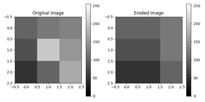
Example of Basic Grayscale Erosion

Following is the example of the function scipy.ndimage.grey_erosion() in which grey scale erosion operation is applied to a simple image without any custom structuring element or iterations −

import numpy as np
import matplotlib.pyplot as plt
from scipy.ndimage import grey_erosion

# Create a synthetic grayscale image
image = np.array([
    [100, 120, 130],
    [80,  200, 150],
    [50,  100, 170]
])

# Apply grayscale erosion with a 2x2 structuring element
eroded_image = grey_erosion(image, size=(2, 2))

# Display original and eroded images
plt.figure(figsize=(8, 4))
plt.subplot(1, 2, 1)
plt.title("Original Image")
plt.imshow(image, cmap='gray', vmin=0, vmax=255)
plt.colorbar()

plt.subplot(1, 2, 2)
plt.title("Eroded Image")
plt.imshow(eroded_image, cmap='gray', vmin=0, vmax=255)
plt.colorbar()

plt.tight_layout()
plt.show()

Here is the output of the function scipy.ndimage.grey_erosion() which is used to implement basic Example of Greyscale erosion −

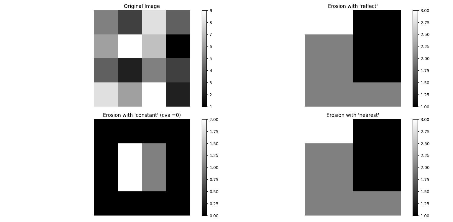
Erosion with Boundary Handling

When performing grey-scale erosion, the mode parameter determines how the boundaries of the input array are handled. This is especially important when the structuring element overlaps the edge of the image. Here's an example of performing grey-scale erosion using the mode parameter to handle boundaries differently −

import numpy as np
import matplotlib.pyplot as plt
from scipy.ndimage import grey_erosion

# Create a simple 2D array (image)
image = np.array([[5, 3, 8, 4],
                  [6, 9, 7, 1],
                  [4, 2, 5, 3],
                  [8, 6, 9, 2]])

# Define a structuring element size
size = (3, 3)

# Apply grey erosion with different boundary modes
erosion_reflect = grey_erosion(image, size=size, mode='reflect')
erosion_constant = grey_erosion(image, size=size, mode='constant', cval=0)
erosion_nearest = grey_erosion(image, size=size, mode='nearest')

# Plot original image and results
plt.figure(figsize=(12, 8))

plt.subplot(2, 2, 1)
plt.title("Original Image")
plt.imshow(image, cmap='gray', interpolation='nearest')
plt.colorbar()
plt.axis('off')

plt.subplot(2, 2, 2)
plt.title("Erosion with 'reflect'")
plt.imshow(erosion_reflect, cmap='gray', interpolation='nearest')
plt.colorbar()
plt.axis('off')

plt.subplot(2, 2, 3)
plt.title("Erosion with 'constant' (cval=0)")
plt.imshow(erosion_constant, cmap='gray', interpolation='nearest')
plt.colorbar()
plt.axis('off')

plt.subplot(2, 2, 4)
plt.title("Erosion with 'nearest'")
plt.imshow(erosion_nearest, cmap='gray', interpolation='nearest')
plt.colorbar()
plt.axis('off')

plt.tight_layout()
plt.show()

Here is the output of the function scipy.ndimage.grey_erosion() which is used to implement Greyscale erosion with different modes −

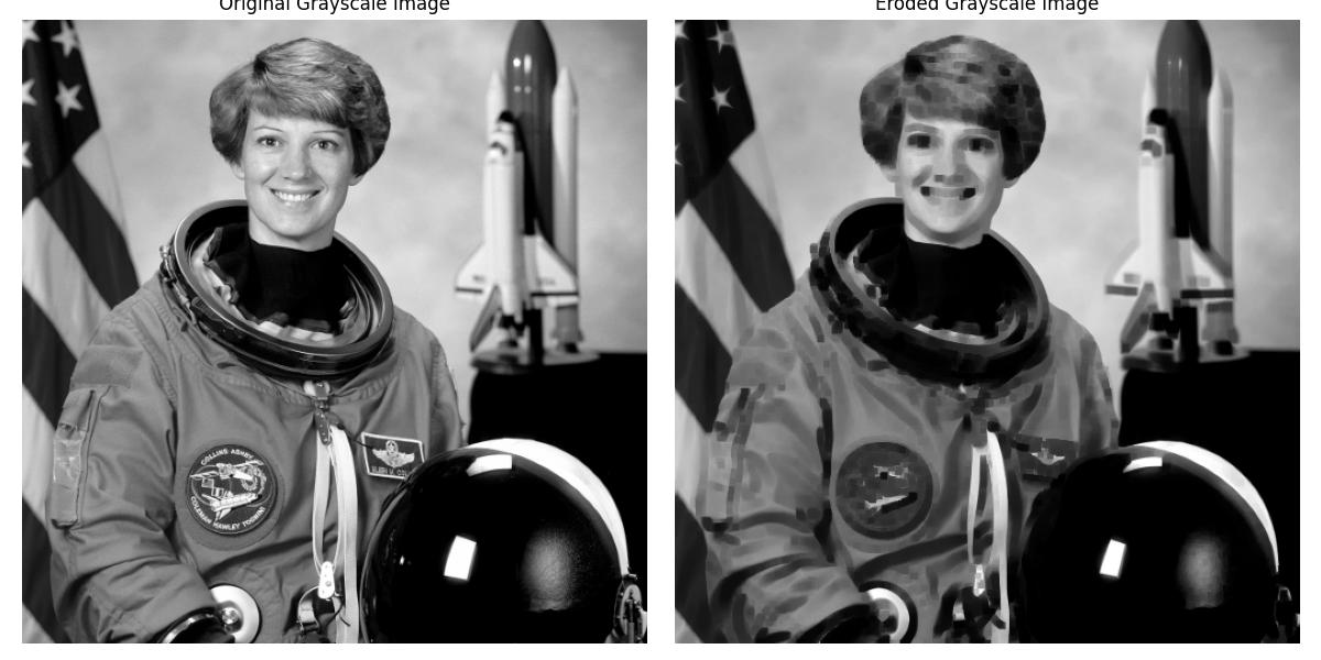
Applying Erosion to Real-World Grayscale Image

In this example we'll apply grey-scale erosion to an image to illustrate its effect. We will use a real-world image from the skimage library and perform grey erosion with a square structuring element −

import numpy as np
import matplotlib.pyplot as plt
from scipy.ndimage import grey_erosion
from skimage import data, color

# Load a sample real-world grayscale image (convert to grayscale if needed)
image = color.rgb2gray(data.astronaut())  # Astronaut image from skimage library
image = (image * 255).astype(np.uint8)  # Scale to 0-255

# Define structuring element size for erosion
size = (5, 5)

# Apply grey erosion
eroded_image = grey_erosion(image, size=size, mode='reflect')

# Plot original and eroded images
plt.figure(figsize=(12, 6))

plt.subplot(1, 2, 1)
plt.title("Original Grayscale Image")
plt.imshow(image, cmap='gray')
plt.axis('off')

plt.subplot(1, 2, 2)
plt.title("Eroded Grayscale Image")
plt.imshow(eroded_image, cmap='gray')
plt.axis('off')

plt.tight_layout()
plt.show()

Here is the output of the function scipy.ndimage.grey_erosion() which is used to implement Greyscale erosion applied to a real image −