SciPy - ndimage.laplace() Function

The scipy.ndimage.laplace() is a function in SciPys ndimage module that applies the Laplacian filter to an image or array. The Laplacian filter computes the second spatial derivative by emphasizing regions of rapid intensity change such as edges.

This function works with N-dimensional arrays and supports different boundary handling modes such as reflect, constant, nearest, mirror, wrap. The cval parameter defines the value used for padding if constant mode is chosen. The output is a new array highlighting edges or intensity variations by making it useful in edge detection and feature extraction tasks in image processing.

Syntax

Following is the syntax of the function scipy.ndimage.laplace() to apply laplace filter on an image −

scipy.ndimage.laplace(input, output=None, mode='reflect', cval=0.0)

Parameters

Following are the parameters of the scipy.ndimage.laplace() function −

• input (array_like): The input image or array on which the Laplace filter will be applied.
• output (array or dtype, optional): The array in which to store the result. If None which is default value then a new array will be created to store the output.
• mode (str, optional): This parameter determines how the input array is extended beyond its boundaries. This affects how the Laplace filter handles edge pixels. The available modes are as follows −
  • reflect: Reflects the input array at the borders. The first pixel value is mirrored. This is the default value.
  • constant: Pads with a constant value which can be specified by cval.
  • nearest: Pads with the nearest boundary value.
  • mirror: This is similar to reflect but mirrors the values at the center of the last pixel.
  • wrap: This parameter wraps the array from the opposite side.
• cval (scalar, optional): The constant value used when mode='constant'. This value will be used to pad the edges of the image when it goes out of bounds. Default value is 0.0.

Return Value

The scipy.ndimage.laplace() function returns the filtered array with the same shape as the input.

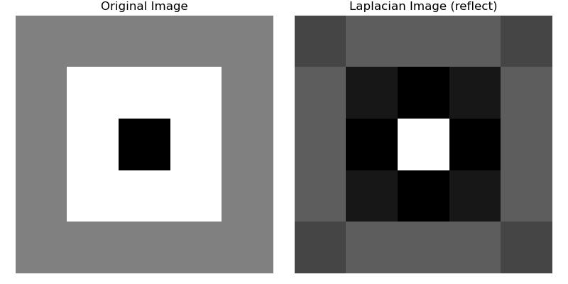
Basic Laplacian Filter Example

Following is the basic example which shows how to use the scipy.ndimage.laplace() function on an image to apply Laplace filter −

import numpy as np
from scipy import ndimage
import matplotlib.pyplot as plt

# Create a 5x5 image
image = np.array([[1, 1, 1, 1, 1],
                  [1, 2, 2, 2, 1],
                  [1, 2, 0, 2, 1],
                  [1, 2, 2, 2, 1],
                  [1, 1, 1, 1, 1]])

# Apply Laplacian filter with default mode ('reflect')
laplacian = ndimage.laplace(image)

# Display the original and Laplacian image
plt.figure(figsize=(8, 4))

plt.subplot(1, 2, 1)
plt.title("Original Image")
plt.imshow(image, cmap='gray')
plt.axis('off')

plt.subplot(1, 2, 2)
plt.title("Laplacian Image (reflect)")
plt.imshow(laplacian, cmap='gray')
plt.axis('off')

plt.tight_layout()
plt.show()

Here is the output of the scipy.ndimage.laplace() function −

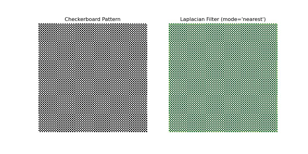
Laplacian Filter with mode='nearest'

This example shows the effect of applying the Laplacian filter with mode='nearest' which handles the boundaries of the image by replicating the nearest values at the edges −

import numpy as np
import matplotlib.pyplot as plt
from scipy import ndimage

# Create a synthetic checkerboard pattern
x = np.indices((100, 100)).sum(axis=0) % 2
image = x.astype(float)

# Apply the Laplacian filter with mode='nearest'
laplacian_nearest = ndimage.laplace(image, mode='nearest')

# Plot
plt.figure(figsize=(10, 5))
plt.subplot(1, 2, 1)
plt.title("Checkerboard Pattern")
plt.imshow(image, cmap='gray')
plt.axis('off')

plt.subplot(1, 2, 2)
plt.title("Laplacian Filter (mode='nearest')")
plt.imshow(laplacian_nearest, cmap='YlGn')
plt.axis('off')

plt.show()

Here is the output of the scipy.ndimage.laplace() function using the mode = 'nearest' −

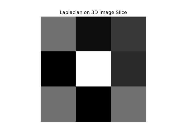
Multi-Dimensional Example with axis=-1

The Laplacian filter can be applied to a 3D or higher-dimensional array. The axis=-1 parameter applies the filter to the last axis of the array which is typically the "depth" axis in a 3D array. Following is the example of using the laplace filter on multi-dimensional image −

import numpy as np
import matplotlib.pyplot as plt
from scipy import ndimage

# Create a 3D array (e.g., 3x3x3)
image_3d = np.array([[[1, 1, 1], [1, 2, 2], [1, 1, 1]],
                     [[1, 2, 2], [2, 0, 2], [1, 2, 1]],
                     [[1, 1, 1], [1, 2, 2], [1, 1, 1]]])

# Apply Laplacian to the last axis (default)
laplacian_3d = ndimage.laplace(image_3d)

# Visualizing a slice of the 3D result
plt.imshow(laplacian_3d[1], cmap='gray')
plt.title("Laplacian on 3D Image Slice")
plt.axis('off')
plt.show()

Here is the output of the scipy.ndimage.laplace() function applied on multidimensional image −