SciPy - signal.firwin2() Function

scipy.signal.firwin2() is a function in SciPy's signal processing module that designs Finite Impulse Response (FIR) filters with arbitrary magnitude frequency responses. It allows users to specify the desired frequency response at specific frequencies and interpolates to construct the filter coefficients.

This function is particularly useful when designing filters that do not fit standard types like low-pass, high-pass or band-pass or when we need custom responses over specific frequency ranges.

Syntax

Following is the syntax for the scipy.signal.firwin2() function which is used to design Finite Impulse Response(FIR) −

scipy.signal.firwin2(numtaps, freq, gain, nfreqs=None, window='hamming', nyq=None, antisymmetric=False, fs=2.0)

Parameters

Here are the parameters of the scipy.signal.firwin2() function which is used to design custom FIR filters −

• numtaps: The number of filter taps (coefficients) in the FIR filter. Must be odd for filters with a symmetric response.
• freq: A sequence of frequency points (normalized or in Hz, based on fs) at which the filters gain is specified.
• gain: A sequence of gain values corresponding to the frequencies in freq. The gain values are interpolated to design the filter.
• nfreqs (optional): Number of frequency points to use in the interpolation. Default value is sufficient for most cases.
• window (optional): Specifies the window function to use for filter design. Default value is 'hamming'.
• nyq (optional): This parameter is Deprecated and we can use fs to specify the sampling frequency.
• antisymmetric (optional): If True then produces a Type III or Type IV linear-phase FIR filter (odd or even length) with an antisymmetric impulse response.
• fs (optional): Sampling frequency of the signal. Default value is 2.0 i.e., normalized frequency.

Return Value

The scipy.signal.firwin2() function returns a 1D array containing the FIR filter coefficients.

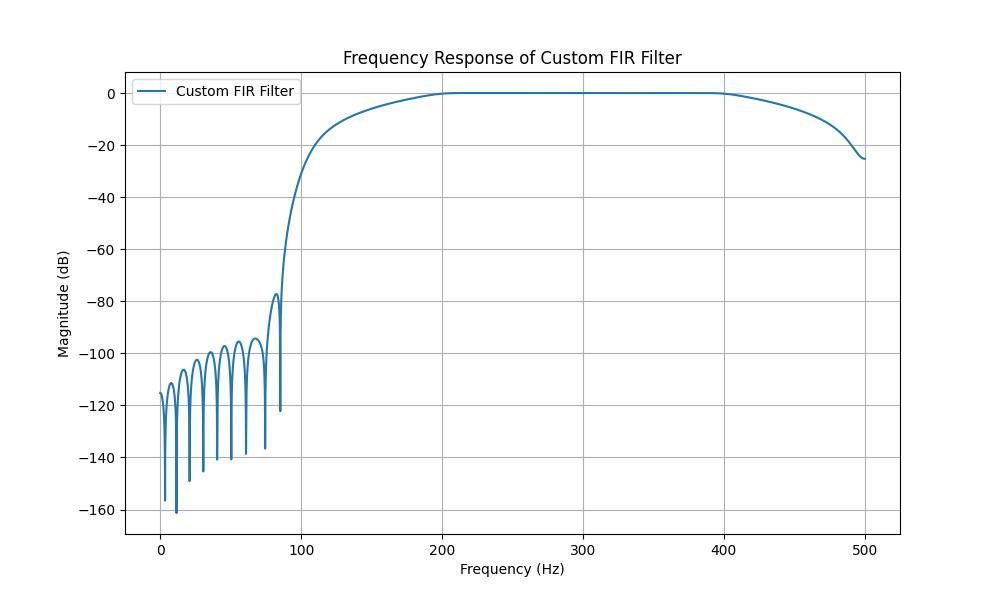
Designing a Custom Filter

Designing a custom FIR filter involves specifying the desired frequency response using the freq and gain parameters. Here is an example of designing a filter with custom response using scipy.signal.firwin2() function −

import numpy as np
from scipy.signal import firwin2, freqz
import matplotlib.pyplot as plt

# Parameters
numtaps = 101  # Number of filter coefficients (should be odd for symmetry)
fs = 1000      # Sampling frequency in Hz
freq = [0, 100, 200, 400, 500]  # Frequency points in Hz (start at 0, end at Nyquist)
gain = [0, 0, 1, 1, 0]          # Desired gain at the corresponding frequency points

# Design custom FIR filter using firwin2
coefficients = firwin2(numtaps, freq, gain, fs=fs)

# Frequency response
w, h = freqz(coefficients, worN=8000, fs=fs)

# Plot the frequency response
plt.figure(figsize=(10, 6))
plt.plot(w, 20 * np.log10(np.abs(h)), label='Custom FIR Filter')
plt.title('Frequency Response of Custom FIR Filter')
plt.xlabel('Frequency (Hz)')
plt.ylabel('Magnitude (dB)')
plt.grid()
plt.legend()
plt.show()

Below is the output of designing a custom FIR filter with the help of scipy.signal.firwin2() function −

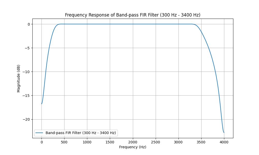
Band-Pass Filter for Audio Frequencies

A band-pass filter allows a certain range of frequencies to pass through while attenuating frequencies outside this range. For audio signals, a typical band-pass filter might pass frequencies from 20 Hz to 20 kHz (the standard human hearing range) or we can design a filter to allow any specific band of frequencies. In this example let's design a simple band-pass FIR filter that passes frequencies between 500 Hz and 5000 Hz which is a common frequency range for many audio applications.

import numpy as np
from scipy.signal import firwin2, freqz
import matplotlib.pyplot as plt

# Parameters
numtaps = 101   # Number of filter coefficients (odd for linear phase)
fs = 8000       # Sampling frequency in Hz (common for speech processing)
lowcut = 300    # Lower cutoff frequency in Hz
highcut = 3400  # Upper cutoff frequency in Hz

# Frequency points (normalized to Nyquist frequency fs/2)
freq = [0, lowcut, highcut, fs/2]  # Frequency breakpoints
gain = [0, 1, 1, 0]  # Corresponding gain at those frequencies

# Design band-pass FIR filter using firwin2
coefficients = firwin2(numtaps, freq, gain, fs=fs)

# Frequency response
w, h = freqz(coefficients, worN=8000, fs=fs)

# Plot the frequency response
plt.figure(figsize=(10, 6))
plt.plot(w, 20 * np.log10(np.abs(h)), label='Band-pass FIR Filter (300 Hz - 3400 Hz)')
plt.title('Frequency Response of Band-pass FIR Filter (300 Hz - 3400 Hz)')
plt.xlabel('Frequency (Hz)')
plt.ylabel('Magnitude (dB)')
plt.grid()
plt.legend()
plt.show()

Following is the output of designing a Band pass filter with the help of scipy.signal.firwin2() function −

High-Pass Filter with Smooth Transition

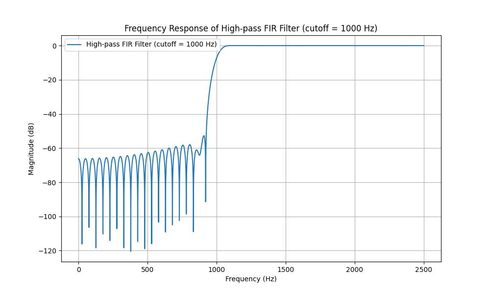
Here in this example we will design a high-pass filter with a smooth transition using scipy.signal.firwin2() function. This type of filter will allow high frequencies to pass through while attenuating the lower frequencies. The transition between passband and stopband should be smooth and can be achieved by selecting appropriate filter parameters −

import numpy as np
from scipy.signal import firwin2, freqz
import matplotlib.pyplot as plt

# Parameters
numtaps = 101  # Number of filter coefficients (odd for linear phase)
fs = 5000      # Sampling frequency in Hz (for demonstration)
cutoff = 1000  # Cutoff frequency in Hz (for high-pass filter)

# Frequency points (normalized to Nyquist frequency fs/2)
freq = [0, cutoff, cutoff, fs/2]  # Frequency breakpoints
gain = [0, 0, 1, 1]  # Gain values at corresponding frequencies

# Design high-pass FIR filter using firwin2
coefficients = firwin2(numtaps, freq, gain, fs=fs)

# Frequency response
w, h = freqz(coefficients, worN=8000, fs=fs)

# Plot the frequency response
plt.figure(figsize=(10, 6))
plt.plot(w, 20 * np.log10(np.abs(h)), label='High-pass FIR Filter (cutoff = 1000 Hz)')
plt.title('Frequency Response of High-pass FIR Filter (cutoff = 1000 Hz)')
plt.xlabel('Frequency (Hz)')
plt.ylabel('Magnitude (dB)')
plt.grid()
plt.legend()
plt.show()

Following is the output of designing a High pass filter with the help of scipy.signal.firwin2() function −