SciPy - signal.firwin() Function

scipy.signal.firwin() is a function in SciPy's signal processing module that designs Finite Impulse Response (FIR) filters using the window method. It creates a filter with the desired frequency response by specifying the cutoff frequencies and other parameters.

This function is useful for constructing low-pass, high-pass, band-pass and band-stop filters for signal processing tasks. By using different windowing techniques we can control the trade-off between the filter's sharpness and ripple.

Syntax

The syntax for the scipy.signal.firwin() function is as follows −

scipy.signal.firwin(numtaps, cutoff, width=None, window='hamming', pass_zero=True, scale=True, nyq=None, fs=2.0)

Parameters

Here are the parameters of the scipy.signal.firwin() function which is used to design FIR filters −

• numtaps: The number of filter taps (coefficients) in the FIR filter. Must be odd for certain filters like band-pass.
• cutoff: The cutoff frequency or frequencies of the filter. For a single frequency which specify a scalar. For band-pass or band-stop, provide a sequence.
• width(optional): Transition width for the filter. Only used for certain window types. If not specified then the default depends on the window.
• window(optional): This parameter specifies the window function used for filter design. Default value is 'hamming'.
• pass_zero(optional): Determines the type of filter. True for low-pass or high-pass and False for band-pass or band-stop.
• scale(optional): If True then the filter coefficients are scaled to ensure unity gain at a certain frequency. Default value is True.
• nyq(optional): This parameter is deprecated. Nyquist frequency of the signal and we can use fs instead.
• fs(optional): Sampling frequency of the signal. Default value is 2.0.

Return Value

The scipy.signal.firwin() function returns a 1D array containing the FIR filter coefficients.

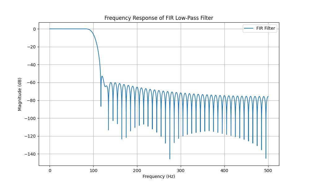
Designing a Low-Pass Filter

Designing a low-pass filter involves selecting parameters that meet specific requirements for attenuating high-frequency components while preserving low-frequency signals. Here is an example of designing a low-pass FIR filter using scipy.signal.firwin() function −

import numpy as np
from scipy.signal import firwin, freqz
import matplotlib.pyplot as plt

# Design a low-pass filter
numtaps = 101
cutoff = 0.3  # Normalized frequency
coefficients = firwin(numtaps, cutoff)

# Plot the frequency response
w, h = freqz(coefficients)
plt.plot(w / np.pi, 20 * np.log10(abs(h)))
plt.title('Low-Pass Filter Frequency Response')
plt.xlabel('Normalized Frequency ( rad/sample)')
plt.ylabel('Magnitude (dB)')
plt.grid()
plt.show()

Following is the output of the designing a low pass filter with the help of scipy.signal.firwin() function −

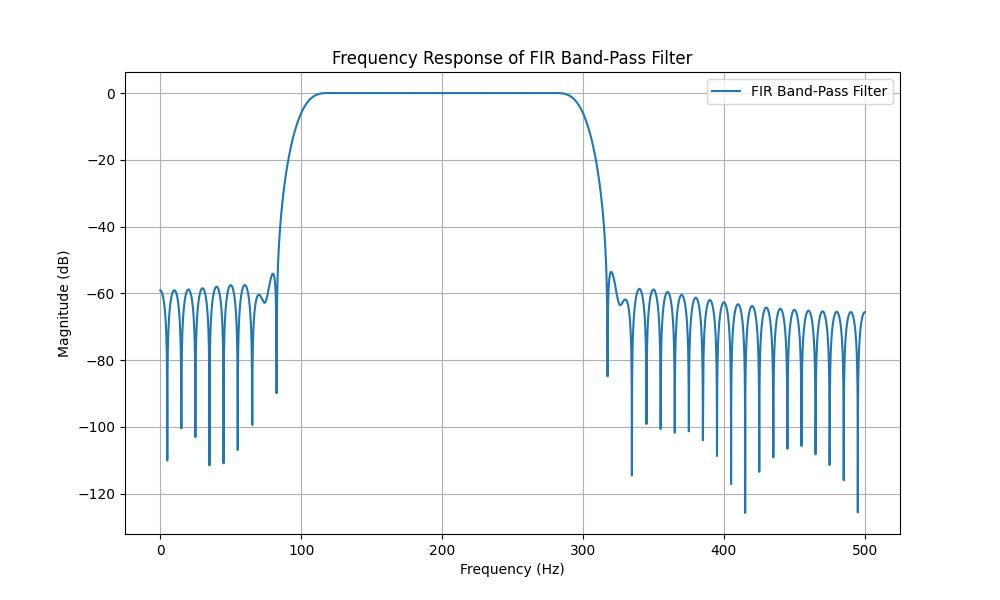
Designing a Band-Pass Filter

A band-pass filter allows frequencies within a specific range i.e., passband to pass through while attenuating frequencies outside this range. This can be achieved using either FIR or IIR filter design methods. Following is the example of designing a Band pass Filter by using the function scipy.signal.firwin() −

import numpy as np
from scipy.signal import firwin, freqz, lfilter
import matplotlib.pyplot as plt

# Parameters
fs = 1000  # Sampling frequency in Hz
low_cutoff = 100  # Low cutoff frequency in Hz
high_cutoff = 300  # High cutoff frequency in Hz
numtaps = 101  # Filter order + 1 (number of coefficients)

# Design FIR band-pass filter
fir_coeff = firwin(numtaps, [low_cutoff, high_cutoff], fs=fs, pass_zero=False)

# Frequency response
w, h = freqz(fir_coeff, worN=8000, fs=fs)

# Plot the frequency response
plt.figure(figsize=(10, 6))
plt.plot(w, 20 * np.log10(np.abs(h)), label='FIR Band-Pass Filter')
plt.title('Frequency Response of FIR Band-Pass Filter')
plt.xlabel('Frequency (Hz)')
plt.ylabel('Magnitude (dB)')
plt.grid()
plt.legend()
plt.show()

Here is the output of the designing a Band pass filter with the help of scipy.signal.firwin() function −

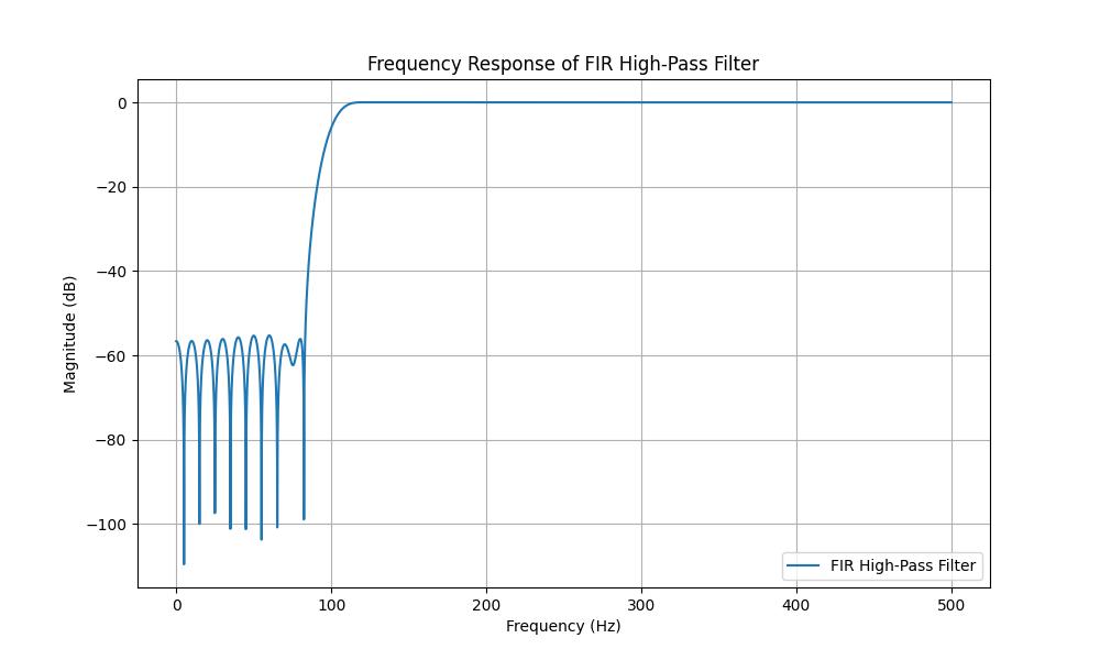
Designing a High-Pass Filter

A high-pass filter allows frequencies above a specified cutoff frequency (f_c) to pass while attenuating frequencies below (f_c). High-pass filters can be implemented as either FIR (Finite Impulse Response) or IIR (Infinite Impulse Response) filters depending on the application and constraints. Here is the example of designing a High-Pass filter −

import numpy as np
from scipy.signal import firwin, freqz, lfilter
import matplotlib.pyplot as plt

# Parameters
fs = 1000  # Sampling frequency in Hz
fc = 100   # Cutoff frequency in Hz
numtaps = 101  # Filter order + 1 (number of coefficients)

# Design FIR high-pass filter
fir_coeff = firwin(numtaps, fc, fs=fs, pass_zero=False)

# Frequency response
w, h = freqz(fir_coeff, worN=8000, fs=fs)

# Plot the frequency response
plt.figure(figsize=(10, 6))
plt.plot(w, 20 * np.log10(np.abs(h)), label='FIR High-Pass Filter')
plt.title('Frequency Response of FIR High-Pass Filter')
plt.xlabel('Frequency (Hz)')
plt.ylabel('Magnitude (dB)')
plt.grid()
plt.legend()
plt.show()

Below is the output of the designing a High pass filter with the help of scipy.signal.firwin() function −