SciPy - signal.kaiserord() Function

Signal kaiserord() Function in SciPy

The scipy.signal.kaiserord() is a function in SciPy's signal processing module that estimates the filter order and Kaiser window parameter for a Finite Impulse Response (FIR) filter. It is useful when designing FIR filters using the Kaiser window method, which offers flexibility in controlling the trade-off between transition width and ripple.

The Kaiser window provides an adjustable parameter, , which allows for better control of the filter's side-lobe attenuation and main-lobe width.

Syntax

The syntax for the scipy.signal.kaiserord() function is as follows −

scipy.signal.kaiserord(ripple, width)

Parameters

Here are the parameters of the scipy.signal.kaiserord() function used to estimate the filter order and window shape parameter −

• ripple: The maximum allowable passband or stopband ripple in decibels (dB).
• width: The transition width of the filter in normalized frequency (0 to 1 range, where 1 represents the Nyquist frequency).

Return Value

The scipy.signal.kaiserord() function returns two values −

• numtaps: The estimated filter order (number of taps required).
• beta: The Kaiser window parameter used for designing the filter.

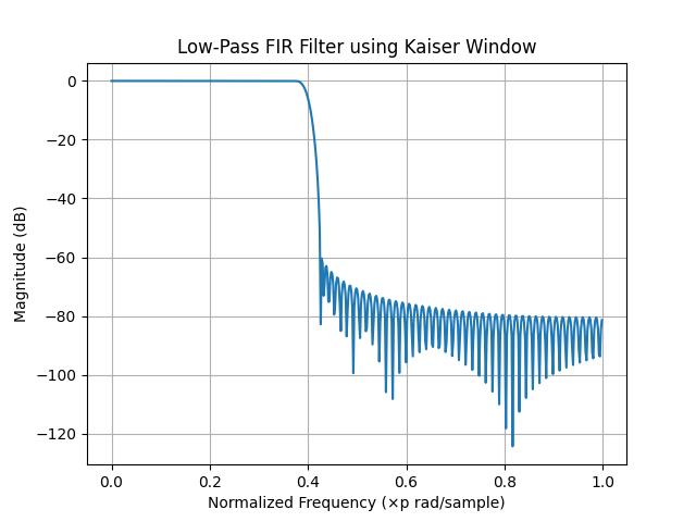
Designing a Low-Pass Filter

Designing a low-pass FIR filter using the Kaiser window involves first determining the required filter order and window parameter using the scipy.signal.kaiserord() function.

Here is an example of designing a low-pass FIR filter using the Kaiser window method −

import numpy as np
from scipy.signal import kaiserord, firwin, freqz
import matplotlib.pyplot as plt

# Desired specifications
ripple = 60  # Maximum ripple in dB
width = 0.05  # Transition width in normalized frequency

# Compute filter order and Kaiser window parameter
numtaps, beta = kaiserord(ripple, width)

# Design the FIR low-pass filter
cutoff = 0.4  # Normalized cutoff frequency
coefficients = firwin(numtaps, cutoff, window=('kaiser', beta))

# Compute frequency response
w, h = freqz(coefficients)

# Plot the frequency response
plt.plot(w / np.pi, 20 * np.log10(abs(h)))
plt.title('Low-Pass FIR Filter using Kaiser Window')
plt.xlabel('Normalized Frequency ( rad/sample)')
plt.ylabel('Magnitude (dB)')
plt.grid()
plt.show()

Below is the output of designing a low-pass FIR filter using the Kaiser window −

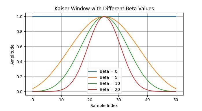
Choosing Kaiser Window Parameters

The Kaiser window provides an adjustable parameter that allows for control over the trade-off between the filter's main-lobe width and side-lobe attenuation. Higher values provide greater attenuation at the cost of a wider main lobe.

Here is an example of visualizing the effect of different Kaiser window parameters −

import numpy as np
import matplotlib.pyplot as plt
from scipy.signal import kaiser

# Define window lengths and beta values
N = 51
beta_values = [0, 5, 10, 20]

# Plot Kaiser windows for different beta values
plt.figure(figsize=(10, 6))
for beta in beta_values:
    window = kaiser(N, beta)
    plt.plot(window, label=f'Beta = {beta}')

plt.title('Kaiser Window with Different Beta Values')
plt.xlabel('Sample Index')
plt.ylabel('Amplitude')
plt.legend()
plt.grid()
plt.show()

Below is the output of visualizing the Kaiser window for different values −