SciPy - stats.norm.pdf() Function

---

---

scipy.stats.norm.pdf() is a function in SciPy that computes the probability density function (PDF) of a normal (Gaussian) distribution at a given value x. This function is part of SciPys stats module where loc represents the mean () and scale is the standard deviation ().

The mathematical formula used to compute the probability density function is defined as follows −

f(x) = ⁄σ √2π e^{- ⁄ (x - μ)2 / 2σ2}

Syntax

Following is the syntax of the function scipy.stats.norm.pdf() which computes the probability density function −

scipy.stats.norm.pdf(x, loc=0, scale=1)

Parameters

Below are the parameters of the scipy.stats.norm.pdf() function −

• x: The value at which the PDF is evaluated.
• loc (optional): The mean () of the normal distribution. Default value is 0.
• scale (optional): The standard deviation () of the normal distribution. Default value is 1.

Return Value

The scipy.stats.norm.pdf() function returns the probability density function value at x by representing the height of the normal distribution curve at that point.

Example of Standard Normal Distribution

The standard normal distribution is a special case of the normal distribution where the mean () is 0 and the standard deviation () is 1. It is used widely in statistics and probability theory.

In the standard normal distribution, the highest point occurs at x = 0 where the probability density is the largest.

In this example we will compute the probability density at x = 0 for the standard normal distribution by using the scipy.stats.norm.pdf() function −

import numpy as np
from scipy.stats import norm

# Define the parameters for the standard normal distribution
x = 0
mean = 0
std_dev = 1

# Compute the PDF for standard normal distribution
pdf_value = norm.pdf(x, loc=mean, scale=std_dev)

# Print the result
print(f"PDF value at x={x}: {pdf_value}")

Following is the output standard normal distribution computed by using the function scipy.stats.norm.pdf() −

PDF value at x=0: 0.3989422804014327

Example of Normal Distribution

The normal distribution is a continuous probability distribution characterized by its bell-shaped curve. It is defined by its mean () and standard deviation () where the mean determines the center of the distribution and the standard deviation controls the width. The normal distribution is widely used in statistics, finance, and various fields of science.

In this example, we will compute the probability density at a given point (x = 2) for a normal distribution with mean () = 3 and standard deviation () = 2 by using the scipy.stats.norm.pdf() function −

import numpy as np
from scipy.stats import norm

# Define the parameters for the normal distribution
x = 2
mean = 3
std_dev = 2

# Compute the PDF for the normal distribution
pdf_value = norm.pdf(x, loc=mean, scale=std_dev)

# Print the result
print(f"PDF value at x={x}: {pdf_value}")

Below is the output of the normal distribution computed by using the function scipy.stats.norm.pdf() −

PDF value at x=2: 0.17603266338214976

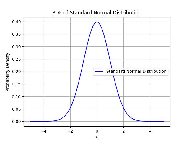
Example of Evaluating PDF for a Range of Values

In this example, we will compute the probability density function for a range of x values between -5 and 5 using the scipy.stats.norm.pdf() function and visualize the distribution curve −

import numpy as np
import matplotlib.pyplot as plt
from scipy.stats import norm

# Define the range of x values
x_values = np.linspace(-5, 5, 100)

# Compute the PDF for each x value
pdf_values = norm.pdf(x_values, loc=0, scale=1)

# Plot the PDF
plt.plot(x_values, pdf_values, label="Standard Normal Distribution", color="blue")
plt.title("PDF of Standard Normal Distribution")
plt.xlabel("x")
plt.ylabel("Probability Density")
plt.legend()
plt.grid(True)
plt.show()

Following is the output of the standard normal distribution computed using the function scipy.stats.norm.pdf() visualized as a probability density curve −