- Generative AI - Home
- Generative AI Basics
- Generative AI Basics
- Generative AI Evolution
- ML and Generative AI
- Generative AI Models
- Discriminative vs Generative Models
- Types of Gen AI Models
- Probability Distribution
- Probability Density Functions
- Maximum Likelihood Estimation
- Generative AI Networks
- How GANs Work?
- GAN - Architecture
- Conditional GANs
- StyleGAN and CycleGAN
- Training a GAN
- GAN Applications
- Generative AI Transformer
- Transformers in Gen AI
- Architecture of Transformers in Gen AI
- Input Embeddings in Transformers
- Multi-Head Attention
- Positional Encoding
- Feed Forward Neural Network
- Residual Connections in Transformers
- Generative AI Autoencoders
- Autoencoders in Gen AI
- Autoencoders Types and Applications
- Implement Autoencoders Using Python
- Variational Autoencoders
- Generative AI and ChatGPT
- A Generative AI Model
- Generative AI Miscellaneous
- Gen AI for Manufacturing
- Gen AI for Developers
- Gen AI for Cybersecurity
- Gen AI for Software Testing
- Gen AI for Marketing
- Gen AI for Educators
- Gen AI for Healthcare
- Gen AI for Students
- Gen AI for Industry
- Gen AI for Movies
- Gen AI for Music
- Gen AI for Cooking
- Gen AI for Media
- Gen AI for Communications
- Gen AI for Photography
Implement Autoencoders Using Python
Autoencoders are a type of artificial neural network (ANN) used to learn efficient coding of unlabeled data. They have become an essential tool in the field of machine learning and deep learning. This chapter provides a step-by-step guide to implement autoencoders in Python programming language. We will use the MNIST dataset for our example.
We will cover the necessary setup, data preprocessing, model building, training, and visualization of the results. We will use MNIST dataset of handwritten digits for our example.
Step-by-Step Guide to Implement Autoencoders Using Python
Lets explore the steps to implement autoencoders using Python programming language −
Step 1: Setting Up the Environment
Before getting started with the implementation, we must ensure that the necessary libraries are installed. If they are not installed, you can use pip command as given below to install them −
pip install numpy matplotlib tensorflow
Step 2: Importing Libraries
Once we done with the installation, we need to import the necessary libraries −
# Import necessary libraries
import numpy as np
import matplotlib.pyplot as plt
from tensorflow.keras.datasets import mnist
from tensorflow.keras.models import Model
from tensorflow.keras.layers import Input, Dense, Flatten, Reshape
from tensorflow.keras.optimizers import Adam
Step 3: Loading and Preprocessing the MNIST Dataset
In this step, we will load the MNIST handwritten digit dataset and normalize the pixel values as follows −
# Load the dataset
(x_train, _), (x_test, _) = mnist.load_data()

# Normalize the data
x_train = x_train.astype('float32') / 255.0
x_test = x_test.astype('float32') / 255.0

# Reshape the data to include the channel dimension
x_train = np.reshape(x_train, (len(x_train), 28, 28, 1))
x_test = np.reshape(x_test, (len(x_test), 28, 28, 1))
Step 4: Building the Autoencoder Model
In this step, we will build the autoencoder model by defining the encoder and decoder parts −
# Define the input shape for the autoencoder
input_shape = (28, 28, 1)

# Define the encoder part of the autoencoder
input_img = Input(shape=input_shape)
x = Flatten()(input_img)
encoded = Dense(64, activation='relu')(x)

# Define the decoder part of the autoencoder
decoded = Dense(784, activation='sigmoid')(encoded)
decoded = Reshape((28, 28, 1))(decoded)

# Define the complete autoencoder model
autoencoder = Model(input_img, decoded)
autoencoder.compile(optimizer=Adam(), loss='binary_crossentropy')

# Print the summary of the autoencoder model
autoencoder.summary()
Step 5: Training the Autoencoder Model
Next, we need to train the autoencoder with the training data as follows −
# Train the autoencoder
autoencoder.fit(x_train, x_train,
   epochs = 50,		# Number of epochs to train
   batch_size=256,	# Batch size for training
   shuffle=True,
   validation_data = (x_test, x_test)
)
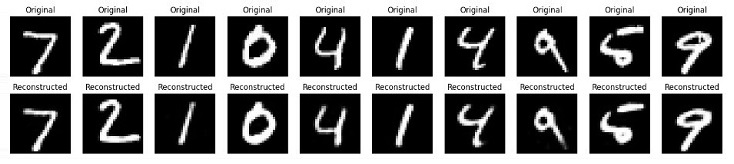
Step 6: Visualizing Original and Reconstructed Data
In this final step, we will visualize some of the original and reconstructed images to check how well the autoencoder has performed.
# Predict the reconstructed images from the test set
decoded_imgs = autoencoder.predict(x_test)

# Number of digits to display
n = 10

# Create a figure with a specified size
plt.figure(figsize=(20, 4))

# Loop through the first n test images

for i in range(n):

   # Display the original image
   ax = plt.subplot(2, n, i + 1)  # Create a subplot for the original image

   # Reshape and plot the original image
   plt.imshow(x_test[i].reshape(28, 28), cmap='gray')
   plt.title("Original")  # Set the title of the plot
   plt.axis('off')

   # Display the reconstructed image
   ax = plt.subplot(2, n, i + 1 + n)
   plt.imshow(decoded_imgs[i].reshape(28, 28), cmap='gray')
   plt.title("Reconstructed")
   plt.axis('off')

# Show the figure
plt.show()
Complete Python Implementation Code
Given below is the complete Python script of above example and its output −
# Import necessary libraries
import numpy as np
import matplotlib.pyplot as plt
from tensorflow.keras.datasets import mnist
from tensorflow.keras.models import Model
from tensorflow.keras.layers import Input, Dense, Flatten, Reshape
from tensorflow.keras.optimizers import Adam

# Load the dataset
(x_train, _), (x_test, _) = mnist.load_data()

# Normalize the data
x_train = x_train.astype('float32') / 255.0
x_test = x_test.astype('float32') / 255.0

# Reshape the data to include the channel dimension
x_train = np.reshape(x_train, (len(x_train), 28, 28, 1))
x_test = np.reshape(x_test, (len(x_test), 28, 28, 1))

# Define the input shape for the autoencoder
input_shape = (28, 28, 1)

# Define the encoder part of the autoencoder
input_img = Input(shape=input_shape)
x = Flatten()(input_img)
encoded = Dense(64, activation='relu')(x)

# Define the decoder part of the autoencoder
decoded = Dense(784, activation='sigmoid')(encoded)
decoded = Reshape((28, 28, 1))(decoded)

# Define the complete autoencoder model
autoencoder = Model(input_img, decoded)

autoencoder.compile(optimizer=Adam(), loss='binary_crossentropy')

# Print the summary of the autoencoder model
autoencoder.summary()

# Train the autoencoder
autoencoder.fit(x_train, x_train,
   epochs=50,  # Number of epochs to train
   batch_size=256,  # Batch size for training
   shuffle=True,
   validation_data=(x_test, x_test)
)

# Predict the reconstructed images from the test set
decoded_imgs = autoencoder.predict(x_test)

# Number of digits to display
n = 10

# Create a figure with a specified size
plt.figure(figsize=(20, 4))

# Loop through the first n test images
for i in range(n):
   # Display the original image
   ax = plt.subplot(2, n, i + 1)
   plt.imshow(x_test[i].reshape(28, 28), cmap='gray')
   plt.title("Original")  # Set the title of the plot
   plt.axis('off')

   # Display the reconstructed image
   ax = plt.subplot(2, n, i + 1 + n)
   plt.imshow(decoded_imgs[i].reshape(28, 28), cmap='gray')
   plt.title("Reconstructed")
   plt.axis('off')

# Show the figure
plt.show()
Output
After running the above script, it will first print the summary of autoencoder model and then the training epochs. At last, we will get the figure that shows the original and reconstructed data.
Model: "functional_1"
| Layer (type) | Output Shape | Param # |
|---|---|---|
| input_layer_3 (InputLayer) | (None, 28, 28, 1) | 0 |
| flatten_3 (Flatten) | (None, 784) | 0 |
| dense_6 (Dense) | (None, 64) | 50, 240 |
| dense_7 (Dense) | (None, 784) | 50, 960 |
| reshape_3 (Reshape) | (None, 28, 28, 1) | 0 |
Total params: 101,200 (395.31 KB)
Trainable params: 101,200 (395.31 KB)
Non-trainable params: 0 (0.00 B)
Conclusion
Autoencoders are powerful tools for unsupervised learning and can be applied to a variety of tasks, such as dimensionality reduction, feature extraction, and image denoising.
In this chapter, we explained how you can implement a simple autoencoder using Python and apply it to the MNIST handwritten dataset. It involved setting up the environment, preprocessing the data, building and training the model, and visualizing the results to evaluate the model's performance.