Mahotas - Eccentricity of an Image

---

---

The eccentricity of an image refers to the measure of how elongated or stretched the shape of an object or region within the image is. It provides a quantitative measure of how how much the shape deviates from a perfect circle.

The eccentricity value ranges between 0 and 1, where −

• 0 − Indicates a perfect circle. Objects with an eccentricity of 0 have the least elongation and are perfectly symmetric.

• Close to 1 − Indicates increasingly elongated shapes. As the eccentricity value approaches 1, the shapes become more elongated and less circular.

Eccentricity of an Image in Mahotas

We can calculate the eccentricity of an image in Mahotas using the 'mahotas.features.eccentricity()' function.

If the eccentricity value is higher, it indicates that the shapes in the image are more stretched or elongated. On the other hand, if the eccentricity value is lower, it indicates that the shapes are closer to being perfect circles or less elongated.

The mahotas.features.eccentricity() function

The eccentricity() function in mahotas helps us measure how stretched or elongated the shapes are in an image. This function takes an image with single channel as input and returns a float point number between 0 and 1.

Syntax

Following is the basic syntax of the eccentricity() function in mahotas −

mahotas.features.eccentricity(bwimage)

Where, 'bwimage' is the input image interpreted as a boolean value.

Example

In the following example, we are finding the eccentricity of an image −

import mahotas as mh
import numpy as np
from pylab import imshow, show
image = mh.imread('nature.jpeg', as_grey = True)
eccentricity= mh.features.eccentricity(image)
print("Eccentricity of the image =", eccentricity)

Output

Output of the above code is as follows −

Eccentricity of the image = 0.8902515127811386

Calculating Eccentricity using Binary Image

To convert a grayscale image into a binary format, we use a technique called thresholding. This process helps us to separate the image into two parts − foreground (white) and background (black).

We do this by picking a threshold value (indicates pixel intensity), which acts as a cutoff point.

Mahotas simplifies this process for us by providing the ">" operator, which allows us to compare pixel values with the threshold value and create a binary image. With the binary image ready, we can now calculate the eccentricity.

Example

Here, we are trying to calculate the eccentricity of a binary image −

import mahotas as mh
image = mh.imread('nature.jpeg', as_grey=True)
# Converting image to binary based on a fixed threshold
threshold = 128
binary_image = image > threshold
# Calculating eccentricity
eccentricity = mh.features.eccentricity(binary_image)
print("Eccentricity:", eccentricity)

Output

After executing the above code, we get the following output −

Eccentricity: 0.7943319646935899

Calculating Eccentricity using the Skeletonization

Skeletonization, also known as thinning, is a process that aims to reduce the shape or structure of an object, representing it as a thin skeleton. We can achieve this using the thin() function in mahotas.

The mahotas.thin() function takes a binary image as input, where the object of interest is represented by white pixels (pixel value of 1) and the background is represented by black pixels (pixel value of 0).

We can calculate the eccentricity of an image using skeletonization by reducing the image to its skeleton representation.

Example

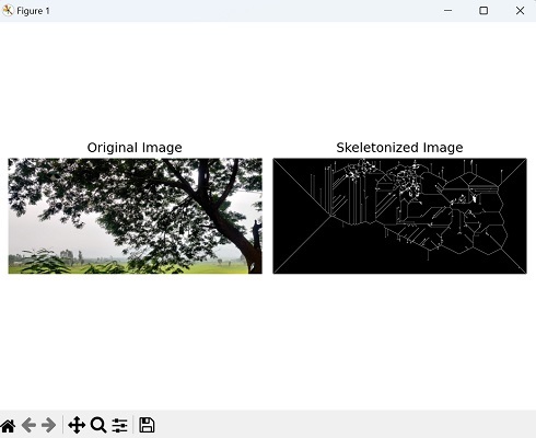
Now, we are calculating the eccentricity of an image using the skeletonization −

import mahotas as mh
import matplotlib.pyplot as plt
# Read the image and convert it to grayscale
image = mh.imread('tree.tiff')
grey_image = mh.colors.rgb2grey(image)
# Skeletonizing the image
skeleton = mh.thin(grey_image)
# Calculating the eccentricity of the skeletonized image
eccentricity = mh.features.eccentricity(skeleton)
# Printing the eccentricity
print(eccentricity)
# Create a figure with subplots
fig, axes = plt.subplots(1, 2, figsize=(7,5 ))
# Display the original image
axes[0].imshow(image)
axes[0].set_title('Original Image')
axes[0].axis('off')
# Display the skeletonized image
axes[1].imshow(skeleton, cmap='gray')
axes[1].set_title('Skeletonized Image')
axes[1].axis('off')
# Adjust the layout and display the plot
plt.tight_layout()
plt.show()

Output

The output obtained is as shown below −

0.8975030064719701

The image displayed is as shown below −