Mahotas - XYZ to LAB Conversion

Quiz

We have discussed about XYZ and LAB color space in our previous tutorial. Now let us discuss about the conversion of XYZ color space to LAB color space.

To convert XYZ to LAB, we need to perform some calculations using specific formulas. These formulas involve adjusting the XYZ values based on a reference white point, which represents a standard for viewing colors.

The adjusted values are then transformed into LAB components using mathematical equations.

In simple terms, the XYZ to LAB conversion allows us to represent colors in a way that aligns better with how our eyes perceive them, making it easier to analyze and compare colors accurately.

XYZ to LAB Conversion in Mahotas

In Mahotas, we can convert an XYZ image to an LAB image using the colors.xyz2lab() function.

The XYZ to LAB conversion in mahotas involves the following steps −

Normalize XYZ values − First, we need to normalize the XYZ values by dividing them by the white point values. The white point represents the reference color that is considered pure white.

This normalization step ensures that the color values are relative to the white point.
Calculate LAB values − Once the XYZ values are normalized, mahotas uses a specific transformation matrix to convert them to LAB. This transformation takes into account the nonlinearities in human color perception and adjust the color values accordingly.
Obtain LAB values − Finally, mahotas provides the LAB values for the color you started with. The resulting LAB values can then be used to describe the color in terms of its lightness and the two color axes.
- L component − The L component in LAB represents the lightness of the color and ranges from 0 to 100. Higher values indicate brighter colors, while lower values indicate darker colors.
- A and B components − The A and B components in LAB represent the color information. The A component ranges from green (-) to red (+), while the B component ranges from blue (-) to yellow (+).
  
  These components provide information about the color characteristics of the XYZ values.

Using the mahotas.colors.xyz2lab() Function

The mahotas.colors.xyz2lab() function takes an XYZ image as input and returns the LAB version of the image.

The resulting LAB image retains the structure and overall content of the original XYZ image but updates the color of each pixel.

Syntax

Following is the basic syntax of the xyz2lab() function in mahotas −

mahotas.colors.xyz2lab(xyz, dtype={float})

where,

xyz − It is the input image in XYZ color space.
dtype (optional − It is the data type of the returned image (default is float).

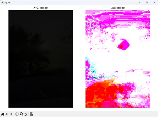
Example

In the following example, we are converting an XYZ image to a LAB image using the mh.colors.xyz2lab() function −

import mahotas as mh
import numpy as np
import matplotlib.pyplot as mtplt
# Loading the image
image = mh.imread('sun.png')
# Converting RGB to XYZ
xyz_image = mh.colors.rgb2xyz(image)
# Converting XYZ to LAB
lab_image = mh.colors.xyz2lab(xyz_image)
# Creating a figure and axes for subplots
fig, axes = mtplt.subplots(1, 2)
# Displaying the XYZ image
axes[0].imshow(xyz_image)
axes[0].set_title('XYZ Image')
axes[0].set_axis_off()
# Displaying the LAB image
axes[1].imshow(lab_image)
axes[1].set_title('LAB Image')
axes[1].set_axis_off()
# Adjusting spacing between subplots
mtplt.tight_layout()
# Showing the figures
mtplt.show()

Output

Following is the output of the above code −

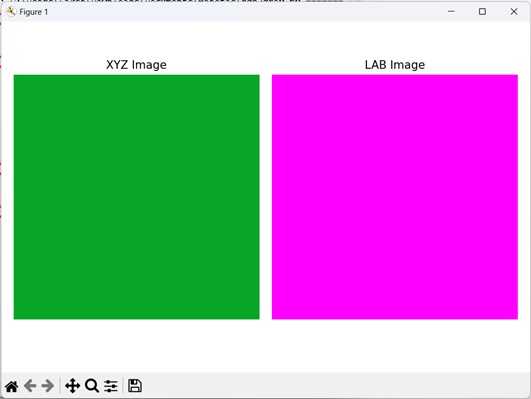
XYZ to LAB Conversion of a Random Image

We can convert a randomly generated XYZ image to LAB color space by first creating an image with any desired dimensions. Next, assign random values to the X, Y, and Z channels for each pixel.

The X, Y, and Z channels represent different color components. Once you have the XYZ image, you can then convert it to an LAB image.

The resulting image will be in the LAB color space with distinct lightness and color channels.

Example

The following example shows conversion of a randomly generated XYZ image to an LAB image −

import mahotas as mh
import numpy as np
import matplotlib.pyplot as mtplt
# Function to create XYZ image
def create_xyz_image(width, height):
   xyz_image = np.zeros((height, width, 3), dtype=np.float32)
   for y in range(height):
      for x in range(width):
         # Assign XYZ values to the pixel
         xyz_image[y, x, 0] = 0.035319468
         xyz_image[y, x, 1] = 0.655582062
         xyz_image[y, x, 2] = 0.157362328
   return xyz_image
# Defining the dimensions of the image
width = 512
height = 512
# Generating the XYZ image
xyz_image = create_xyz_image(width, height)
# Converting XYZ to LAB
lab_image = mh.colors.xyz2lab(xyz_image)
# Creating a figure and axes for subplots
fig, axes = mtplt.subplots(1, 2)
# Displaying the XYZ image
axes[0].imshow(xyz_image)
axes[0].set_title('XYZ Image')
axes[0].set_axis_off()
# Displaying the LAB image
axes[1].imshow(lab_image)
axes[1].set_title('LAB Image')
axes[1].set_axis_off()
# Adjusting spacing between subplots
mtplt.tight_layout()
# Showing the figures
mtplt.show()

Output

Output of the above code is as follows −

Print Page