Mahotas - Wavelet Transforms

---

---

Wavelet transforms are mathematical techniques used to break the images into different frequency components. Wavelet transforms captures both the local and the global details of an image.

Wavelet transforms use small wave−shaped functions, known as wavelets, to analyze signals. These wavelets are scaled and transformed to match different patterns present in an image.

Wavelet transform involves modifying the high and low frequency coefficients of the frequency components to produce identify patterns and enhance and image. The original image can be recovered by inversing the wavelet transform.

Let us discuss about the wavelet transformation techniques along with their inverse variations.

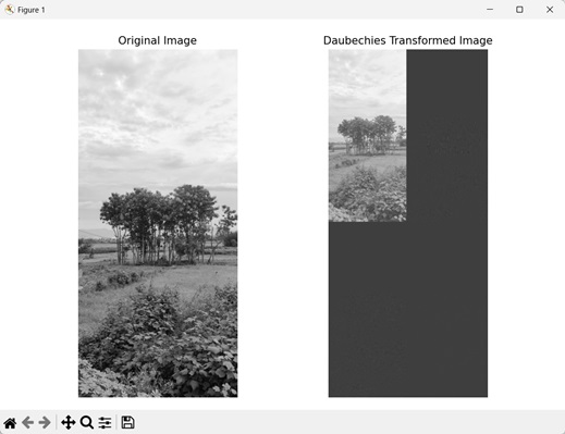
Daubechies Transformation

The Daubechies transformation is a wavelet transformation technique used to break a signal into different frequency components. It allows us to analyze the signals in both the time and the frequency domains.

Let's see Daubechies transformation image below −

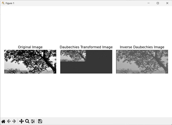
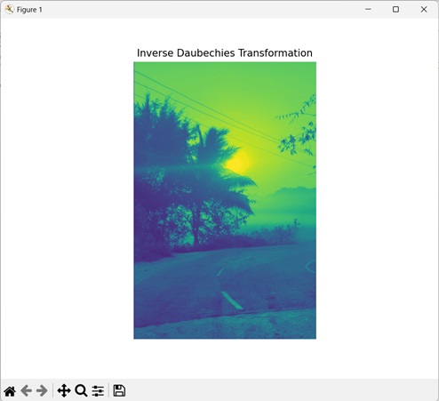
Inverse Daubechies Transformation

The inverse Daubechies transformation is the reverse process of the Daubechies transformation. It reconstructs the original image from the individual frequency components, which are obtained through the Daubechies transformation.

By applying the inverse transform, we can recover the signal while preserving important details.

Here, we look at inverse of Daubechies transformation −

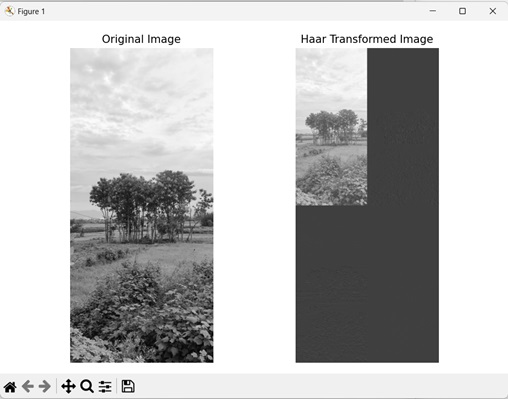
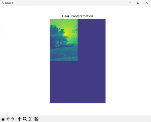
Haar Transformation

The Haar transformation technique breaks down an image into different frequency components by dividing it into sub−regions. It then calculates the difference between the average values to apply wavelet transformation on an image.

In the image below, we see the Haar transformed image −

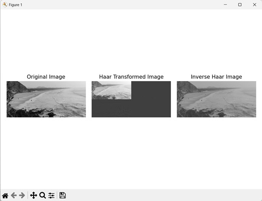
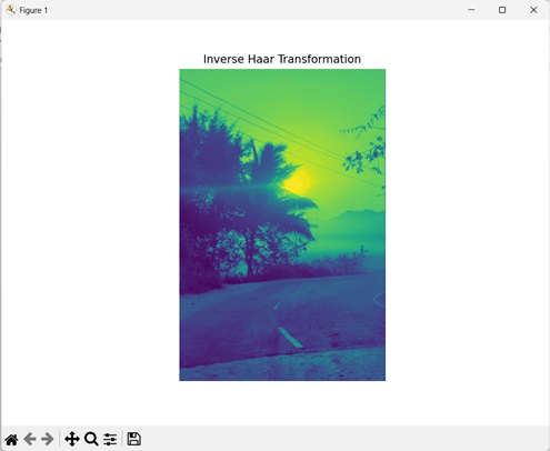
Inverse Haar

The inverse Haar transformation reconstructs the original image from the frequency components obtained through the Haar transformation. It is the reverse operation of the Haar transformation.

Let's look at inverse of Haar transformation −

Example

In the following example, we are trying to perform all the above explained wavelet transformations −

import mahotas as mh
import numpy as np
import matplotlib.pyplot as mtplt
image = mh.imread('sun.png', as_grey=True)
# Daubechies transformation
daubechies = mh.daubechies(image, 'D6')
mtplt.imshow(daubechies)
mtplt.title('Daubechies Transformation')
mtplt.axis('off')
mtplt.show()
# Inverse Daubechies transformation
daubechies = mh.daubechies(image, 'D6')
inverse_daubechies = mh.idaubechies(daubechies, 'D6')
mtplt.imshow(inverse_daubechies)
mtplt.title('Inverse Daubechies Transformation')
mtplt.axis('off')
mtplt.show()
# Haar transformation
haar = mh.haar(image)
mtplt.imshow(haar)
mtplt.title('Haar Transformation')
mtplt.axis('off')
mtplt.show()
# Inverse Haar transformation
haar = mh.haar(image)
inverse_haar = mh.ihaar(haar)
mtplt.imshow(inverse_haar)
mtplt.title('Inverse Haar Transformation')
mtplt.axis('off')
mtplt.show()

Output

The output obtained is as shown below −

Daubechies Transformation:

Inverse Daubechies Transformation:

Haar Transformation:

Inverse Haar Transformation:

We will discuss about all the wavelet transformations in detail in the remaining chapters.