Mahotas - Increase Gamma Correction

---

---

Let us first learn about what is gamma correction before understanding about increase gamma correction.

Gamma correction adjusts the brightness of images to match how our eyes perceive light. Our eyes don't see light in a linear way, so without correction, images may appear too dark or bright.

Gamma correction applies a mathematical transformation to the brightness values, making the image look more natural by adjusting its brightness levels.

Now, increasing gamma correction refers to adjusting the gamma value to make the overall image brighter. When the gamma value is increased, the dark areas appear brighter and enhance the overall contrast of the image.

Increasing Gamma Correction in Mahotas

In Mahotas, increasing gamma correction refers to adjusting the gamma value when changing the brightness of the pixels.

The gamma is a positive value, where −

• A gamma value less than 1 will brighten the image.

• A gamma value greater than 1 will darken the image.

• A gamma value of 1 represents no correction and indicates a linear relationship between the pixel values and luminance.

Gamma correction in Mahotas involves applying a power−law transformation to the intensity values of the image. The power−law transformation is defined as follows −

new_intensity = old_intensity^gamma

Here,

• old_intensity − It is the original intensity value of a pixel

• new_intensity − It is the transformed intensity value after gamma correction.

• The gamma determines the degree of correction applied to the image.

When gamma is increased in Mahotas, it means that the intensity values are raised to a higher power. This adjustment affects the overall brightness of the image.

Mahotas does not provide a direct way to do gamma correction, however it can be achieved by using mahotas with numpy library.

Example

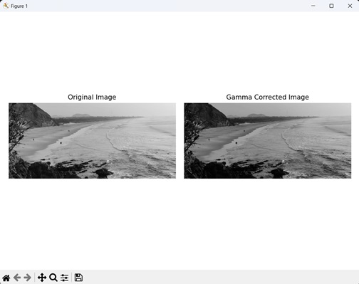
In the following example, we are darkening a grayscale image by decreasing the gamma value −

import mahotas as mh
import numpy as np
import matplotlib.pyplot as mtplt
# Loading the image
image = mh.imread('sea.bmp')
# Converting it to grayscale
gray_image = mh.colors.rgb2gray(image)
# Decreasing gamma value
corrected_gamma = 1.5
# Updating the image to use the corrected gamma value
gamma_correction = np.power(gray_image, corrected_gamma)
# Creating a figure and axes for subplots
fig, axes = mtplt.subplots(1, 2)
# Displaying the original image
axes[0].imshow(gray_image, cmap='gray')
axes[0].set_title('Original Image')
axes[0].set_axis_off()
# Displaying the gamma corrected image
axes[1].imshow(gamma_correction, cmap='gray')
axes[1].set_title('Gamma Corrected Image')
axes[1].set_axis_off()
# Adjusting spacing between subplots
mtplt.tight_layout()
# Showing the figures
mtplt.show()

Output

Following is the output of the above code −

Using Interactive Gamma Correction Slider

An interactive gamma correction slider is a GUI element that allows users to adjust the gamma value dynamically. Users can increase or decrease the gamma value by dragging the slider, providing real−time feedback on the display.

We can increase gamma correction using interactive gamma correction slider in mahotas, by first determining the desired gamma value to increase the correction.

Then, apply the power−law transformation to the image by raising the pixel values to the power of the inverse gamma value.

Syntax

Following is the basic syntax to create an interactive slider −

from matplotlib.widgets import Slider
Slider(slider_axis, name, min_value, max_value, valint)

where,

• slider_axis − It is a list that defines the position and dimensions of the slider.

• name − It is the name of the slider.

• mini_value − It is the minimum value that the slider can go to.

• max_value − It is the maximum value that the slider can go to.

• valint − It is the starting value of the slider.

Example

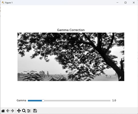
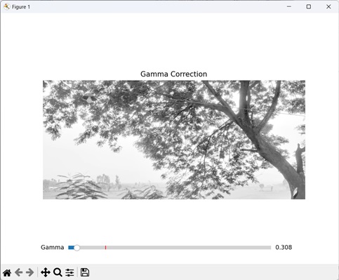
Here, we are trying to increase gamma correction using interactive gamma correction slider −

import mahotas as mh
import numpy as np
import matplotlib.pyplot as mtplt
from matplotlib.widgets import Slider
# Loading the image
image = mh.imread('tree.tiff')
# Converting it to grayscale
image = mh.colors.rgb2gray(image)
# Creating a figure and axes for the plot
fig, axis = mtplt.subplots()
# Displaying the original image
axis.imshow(image, cmap='gray')
axis.set_title('Gamma Correction')
axis.set_axis_off()
# Creating a slider for gamma adjustment
slider_axis = mtplt.axes([0.2, 0.05, 0.6, 0.03])
gamma_slider = Slider(slider_axis, 'Gamma', 0.1, 5.0, valinit=1.0)
# Updating the gamma correction and plot on change of slider value
def update_gamma(val):
   gamma = gamma_slider.val
   corrected_image = np.power(image, gamma)
   axis.imshow(corrected_image, cmap='gray')
   fig.canvas.draw_idle()
gamma_slider.on_changed(update_gamma)
# Showing the figure
mtplt.show()

Output

Output of the above code is as follows. First we are trying to increase the gamma correction using the slider as shown below −

Now, decreasing gamma correction using the slider −

Using Batch Gamma correction

The batch gamma correction applies multiple gamma values to a single image. This helps in comparing the original image side−by−side at different gamma values to see the impact of increasing gamma correction.

In Mahotas, we can adjust the brightness of an image using batch gamma correction by first iterating over a list of predetermined gamma values. Then applying the power−law transformation on the input image with different gamma values.

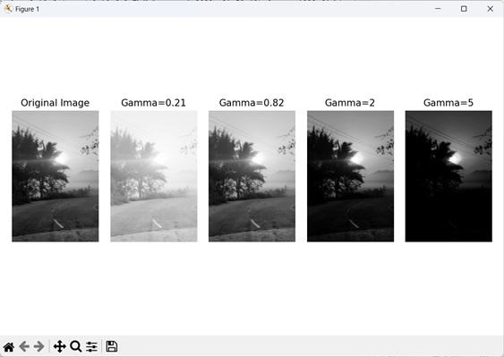
Example

Now, we are trying to increase gamma value using batch gamma correction −

import mahotas as mh
import numpy as np
import matplotlib.pyplot as mtplt
from matplotlib.widgets import Slider
# Loading the image
image = mh.imread('sun.png')
# Converting it to grayscale
image = mh.colors.rgb2gray(image)
# Defining a list of gamma values
gamma_values = [0.21, 0.82, 2, 5]
# Creating subplots to display images for each gamma value
fig, axes = mtplt.subplots(1, len(gamma_values) + 1)
axes[0].imshow(image, cmap='gray')
axes[0].set_title('Original Image')
axes[0].set_axis_off()
# Applying gamma correction for each gamma value
for i, gamma in enumerate(gamma_values):
   corrected_image = np.power(image, gamma)
   axes[i + 1].imshow(corrected_image, cmap='gray')
   axes[i + 1].set_title(f'Gamma={gamma}')
   axes[i + 1].set_axis_off()
# Adjusting spacing between subplots
mtplt.tight_layout()
# Showing the figures
mtplt.show()

Output

Following is the output of the above code −