Mahotas - Making Image Wavelet Center

Quiz

Image wavelet centering refers to shifting the wavelet coefficients of an image to the wavelet center, a point at which the wavelet reaches its maximum amplitude. Wavelet coefficients are numerical values representing the contribution of different frequencies to an image.

Wavelet coefficients are obtained by breaking an image into individual waves using a wavelet transformation. By centering the coefficients, the low and high frequencies can be aligned with the central frequencies to remove noise from an image.

Making Image Wavelet Center in Mahotas

In Mahotas, we can use the mahotas.wavelet_center() function to make an image wavelet centered to reduce noise. The function performs two major steps to make the image wavelet centered, they are as follows −

First it decomposes the signals of the original image into wavelet coefficients.
Next, it takes the approximation coefficients, which are coefficients with low frequencies, and aligns them with central frequencies.

By doing the alignment of frequencies, the average intensity of the image is removed, hence removing noise.

The mahotas.wavelet_center() function

The mahotas.wavelet_center() function takes an image as input, and returns a new image with the wavelet center at the origin.

It decomposes (breaks−down) the original input image using a wavelet transformation and then shifts the wavelet coefficients to the center of the frequency spectrum.

The function ignores a border region of the specified pixel size when finding the image wavelet center.

Syntax

Following is the basic syntax of the wavelet_center() function in mahotas −

mahotas.wavelet_center(f, border=0, dtype=float, cval=0.0)

where,

f − It is the input image.
border (optional) − It is the size of the border area (default is 0 or no border).
dtype (optional) − It is the data type of the returned image (default is float).
cval (optional) − It is the value used to fill the border area (default is 0).

Example

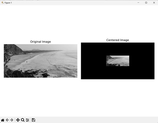
In the following example, we are making an image wavelet centered using the mh.wavelet_center() function.

import mahotas as mh
import numpy as np
import matplotlib.pyplot as mtplt
# Loading the image
image = mh.imread('sun.png')
# Converting it to grayscale
image = mh.colors.rgb2gray(image)
# Centering the image
centered_image = mh.wavelet_center(image)
# Creating a figure and axes for subplots
fig, axes = mtplt.subplots(1, 2)
# Displaying the original image
axes[0].imshow(image, cmap='gray')
axes[0].set_title('Original Image')
axes[0].set_axis_off()
# Displaying the centered image
axes[1].imshow(centered_image, cmap='gray')
axes[1].set_title('Centered Image')
axes[1].set_axis_off()
# Adjusting spacing between subplots
mtplt.tight_layout()
# Showing the figures
mtplt.show()

Output

Following is the output of the above code −

Centering using a Border

We can perform image wavelet centering using a border to manipulate the output image. A border area refers to a region surrounding an object in the image. It separates the object from background region or neighboring objects.

In mahotas, we can define an area that should not be considered when doing wavelet centering by setting the pixel values to zero. This is done by passing a value to the border parameter of the mahotas.wavelet_center() function.

The function ignores as many pixels as specified in the parameter when doing image wavelet centering. For example, if border parameter is set to 500, then 500 pixels on all sides will be ignored when centering the image wavelet.

Example

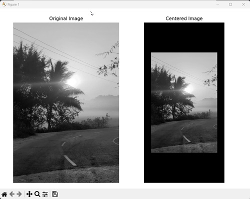
In the example mentioned below, we are ignoring a border of certain size when centering an image wavelet.

import mahotas as mh
import numpy as np
import matplotlib.pyplot as mtplt
# Loading the image
image = mh.imread('sea.bmp')
# Converting it to grayscale
image = mh.colors.rgb2gray(image)
# Centering the image with border
centered_image = mh.wavelet_center(image, border=500)
# Creating a figure and axes for subplots
fig, axes = mtplt.subplots(1, 2)
# Displaying the original image
axes[0].imshow(image, cmap='gray')
axes[0].set_title('Original Image')
axes[0].set_axis_off()
# Displaying the centered image
axes[1].imshow(centered_image, cmap='gray')
axes[1].set_title('Centered Image')
axes[1].set_axis_off()
# Adjusting spacing between subplots
mtplt.tight_layout()
# Showing the figures
mtplt.show()

Output

Output of the above code is as follows −

Centering by applying Padding

We can also do centering by applying padding to fill the border area with a shade of gray.

Padding refers to the technique of adding extra pixel values around the edges of an image to create a border.

In mahotas, padding can be applied by specifying a value to the cval parameter of the mahotas.wavelet_center() function. It allows us to fill the border region with a color, with the value ranging from 0 (black) to 255 (white).

Note − Padding can only be applied if a border area is present. Hence, the value or border parameter should not be 0.

Example

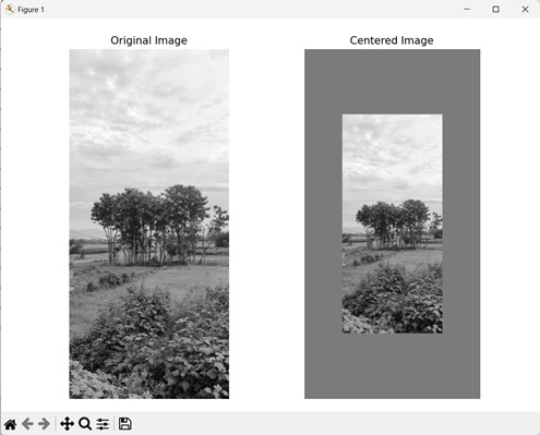
In here, we are ignoring a border of specific pixel size and applying padding to center an image wavelet.

import mahotas as mh
import numpy as np
import matplotlib.pyplot as mtplt
# Loading the image
image = mh.imread('nature.jpeg')
# Converting it to grayscale
image = mh.colors.rgb2gray(image)
# Centering the image with border
centered_image = mh.wavelet_center(image, border=100, cval=109)
# Creating a figure and axes for subplots
fig, axes = mtplt.subplots(1, 2)
# Displaying the original image
axes[0].imshow(image, cmap='gray')
axes[0].set_title('Original Image')
axes[0].set_axis_off()
# Displaying the centered image
axes[1].imshow(centered_image, cmap='gray')
axes[1].set_title('Centered Image')
axes[1].set_axis_off()
# Adjusting spacing between subplots
mtplt.tight_layout()
# Showing the figures
mtplt.show()

Output

After executing the above code, we get the following output −

Print Page