Mahotas - Gaussian Filtering

Quiz

Gaussian filtering is a technique used to blur or smoothen an image. It reduces the noise in the image and softens the sharp edges.

Imagine your image as a grid of tiny dots, and each dot represents a pixel. Gaussian filtering works by taking each pixel and adjusting its value based on the surrounding pixels.

It calculates a weighted average of the pixel values in its neighborhood, placing more emphasis on the closer pixels and less emphasis on the farther ones.

By repeating this process for every pixel in the image, the Gaussian filter blurs the image by smoothing out the sharp transitions between different areas and reducing the noise.

The size of the filter determines the extent of blurring. A larger filter size means a broader region is considered, resulting in more significant blurring.

In simpler terms, Gaussian filtering makes an image look smoother by averaging the nearby pixel values, giving more importance to the closer pixels and less to the ones farther away. This helps to reduce noise and make the image less sharp.

Gaussian Filtering in Mahotas

In Mahotas, we can perform Gaussian filtering on an image using the mahotas.gaussian_filter() function. This function applies a blurring effect to an image by using a special matrix called a Gaussian kernel.

A Gaussian kernel is a special matrix with numbers arranged in a specific way. Each number in the kernel represents a weight.

The kernel is placed over each pixel in the image, and the values of the neighboring pixels are multiplied by their corresponding weights in the kernel.

The multiplied values are then summed, and assigned as the new value to the central pixel. This process is repeated for every pixel in the image, resulting in a blurred image where the sharp details and noise are reduced.

The mahotas.gaussian_filter() function

The mahotas.gaussian_filter() function takes a grayscale image as an input and returns a blurred version of the image as output.

The amount of blurring is determined by the sigma value. The higher the sigma value, more will be the blurring applied to the output image.

Syntax

Following is the basic syntax of the gaussian_filter() function in mahotas −

mahotas.gaussian_filter(array, sigma, order=0, mode='reflect', cval=0.,
out={np.empty_like(array)})

Where,

array − It is the input image.
sigma − It determines the standard deviation of the Gaussian kernel.
order (optional) − It specifies the order of the Gaussian filter. Its value can be 0, 1, 2, or 3 (default is 0).
mode (optional) − It specifies how the border should be handled (default is 'reflect').
cval (optional) − It represents the padding value applied when mode is 'constant'(default is 0).
out (optional) − It specifies where to store the output image (default is an array of same size as array).

Example

In the following example, we are applying Gaussian filtering on an image using the mh.gaussian_filter() function.

import mahotas as mh
import numpy as np
import matplotlib.pyplot as mtplt
# Loading the image
image = mh.imread('tree.tiff')
# Converting it to grayscale
image = mh.colors.rgb2gray(image)
# Applying gaussian filtering
gauss_filter = mh.gaussian_filter(image, 4)
# Creating a figure and axes for subplots
fig, axes = mtplt.subplots(1, 2)
# Displaying the original image
axes[0].imshow(image)
axes[0].set_title('Original Image')
axes[0].set_axis_off()
# Displaying the gaussian filtered image
axes[1].imshow(gauss_filter)
axes[1].set_title('Gaussian Filtered Image')
axes[1].set_axis_off()
# Adjusting spacing between subplots
mtplt.tight_layout()
# Showing the figures
mtplt.show()

Output

Following is the output of the above code −

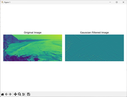
Filtering with Different Order

We can perform Gaussian filtering on an image with different order. Order in Gaussian filtering determines the degree of smoothness (blurring) applied on the image.

Higher the order value, more will be the smoothing effect applied on the image.

Higher orders are useful when dealing with very noisy images. However, higher orders also increase the processing time as the filter is applied multiple times.

An order of 0 applies Gaussian filter once, an order of 1, 2, or 3 applies Gaussian filter twice, thrice and four times respectively.

In mahotas, to perform gaussian filtering with different order, we pass any value other than 0 as the order parameter to the gaussian_filter() function.

Example

In the example mentioned below, we are applying Gaussian filtering on an image with different orders.

import mahotas as mh
import numpy as np
import matplotlib.pyplot as mtplt
# Loading the image
image = mh.imread('sea.bmp')
# Converting it to grayscale
image = mh.colors.rgb2gray(image)
# Applying gaussian filtering
gauss_filter = mh.gaussian_filter(image, 3, 1)
# Creating a figure and axes for subplots
fig, axes = mtplt.subplots(1, 2)
# Displaying the original image
axes[0].imshow(image)
axes[0].set_title('Original Image')
axes[0].set_axis_off()
# Displaying the gaussian filtered image
axes[1].imshow(gauss_filter)
axes[1].set_title('Gaussian Filtered Image')
axes[1].set_axis_off()
# Adjusting spacing between subplots
mtplt.tight_layout()
# Showing the figures
mtplt.show()

Output

Output of the above code is as follows −

Filtering with 'Mirror' Mode

When applying filters to images, it is important to determine how to handle the borders of the image. The mirror mode is a common approach that handles border pixels by mirroring the image content at the borders.

This means that the values beyond the image boundaries are obtained by mirroring the nearest pixels within the image. This is done by mirroring the existing pixels along the edges.

This mirroring technique ensures a smooth transition between the actual image and the mirrored image, resulting in better continuity.

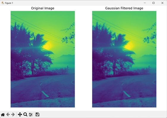
Example

In here, we are applying Gaussian filtering on an image with 'mirror' mode.

import mahotas as mh
import numpy as np
import matplotlib.pyplot as mtplt
# Loading the image
image = mh.imread('sun.png')
# Converting it to grayscale
image = mh.colors.rgb2gray(image)
# Applying gaussian filtering
gauss_filter = mh.gaussian_filter(image, 3, 0, mode='mirror')
# Creating a figure and axes for subplots
fig, axes = mtplt.subplots(1, 2)
# Displaying the original image
axes[0].imshow(image)
axes[0].set_title('Original Image')
axes[0].set_axis_off()
# Displaying the gaussian filtered image
axes[1].imshow(gauss_filter)
axes[1].set_title('Gaussian Filtered Image')
axes[1].set_axis_off()
# Adjusting spacing between subplots
mtplt.tight_layout()
# Showing the figures
mtplt.show()

Output

After executing the above code, we get the following output −

Print Page