Excel - Format Grids

---

Whenever you open the Excel worksheet, gridlines are automatically displayed to separate the rows and columns partitioning each cell, which allows you to read the dataset more clearly. You can also hide these gridlines, which display the worksheet as a single report page similar to an MS Word page. Gridline color, which is Automatic by default, can also be modified in the specific worksheet.

Hide the Gridlines in Microsoft Excel Worksheet

Given below are the steps to hide the gridlines in a specific worksheet −

• You may select the "Sheet5" worksheet in the Microsoft Excel.
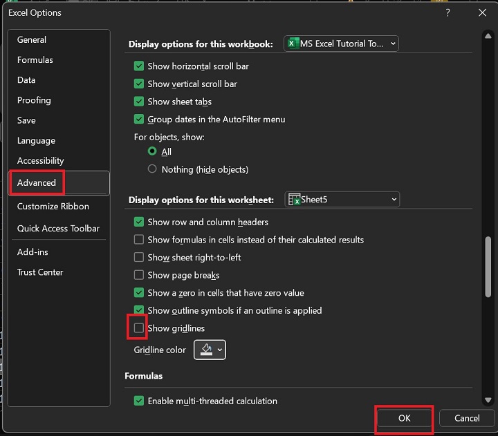
• Click the File tab, select the More category, and then choose the Options from the drop-down menu.

Another "Excel Options" dialog box will appear. You can choose the "Advanced" category and uncheck the "Show gridlines" option in the "Display options for this worksheet". After that, click on the OK button.

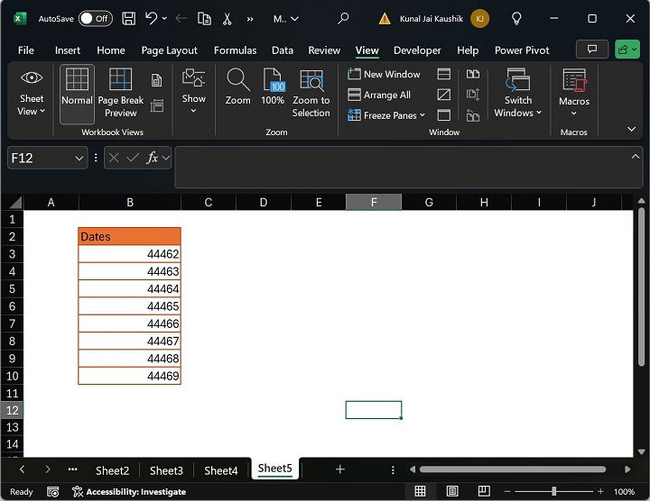
Therefore, the gridlines are hidden in the Microsoft Excel worksheet.

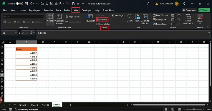
The Alternative way to hide the gridlines in the Microsoft Excel worksheet is to navigate to the "View" tab and deselect the "Gridlines" checkbox under the "Show" group.

Change the Color of Gridlines

You may alter the color of the gridlines only in these Microsoft Excel versions: Excel 2019, Excel 2016, Excel 2021, and Excel for Microsoft 365.

The following steps are written below −

Step 1 − First, make the active worksheet a Sheet 5.

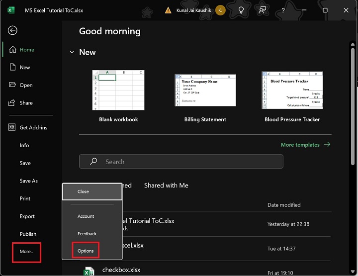
Step 2 − After that, you can choose the File tab and click on the "More" category, and then select "Options" from the menu.

Step 3 − In the "Excel Options" dialog box, you may select the "Advanced" category. Furthermore, expand the "Gridline Color" tile and select the "Sea Green" color from the given list of colors under the "Display options for this worksheet" section. After that, click on the OK button.

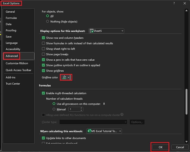
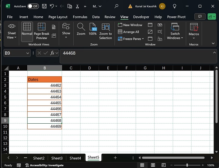
As you can notice in the screenshot, the gridline color has been changed from Automatic to Green.