Excel - Highlight Cell Rules

---

Conditional formatting is a powerful feature that allows you to format cells only after satisfying certain criteria. The Conditional Formatting button provides various options, like Icon Sets, Color Scales, etc. One exclusive option is "Highlight Cells Rules", which allows you to format and highlight cells with vibrant available colors if the condition is true.

The first exclusive option under the Conditional Formatting button is "Highlight Cells Rules" in Microsoft Excel. When you select "Highlight Cells Rules", different rules are displayed in a drop-down menu.

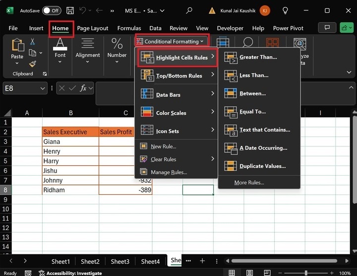
While selecting these cell rules, the different colors can be chosen to highlight the cell values given below −

• Red Text
• Light Right Fill with Dark Red Text
• Red Border
• Yellow Fill with Dark Yellow Text
• Green Fill with Dark Green Text
• Light Red Fill

Types of Cell Rules

Various types of cell rules are listed below −

• Greater Than...(>)
• Less Than..(<)
• Between…
• Equal To…(=)
• Text that Contains…
• A Date Occurring…
• Duplicate Values…

Lets discuss each rule thoroughly −

• Greater Than…(>) − You can choose the "Greater Than…" cell rule to highlight only those values that exceed the specified number in the condition.
• Less Than…(<) − You can set the "Less Than" rules in case of highlighting those cells that are less than the specified in the condition.
• Between… − This rule can be chosen to highlight cell values that lie between two numbers specified in the condition.
• Equal To(=) − This rule formats only those cells equal to the specified number defined in the condition.
• Text that Contains… − This rule highlights only those cells that comprise the text.
• A Date Occurring… − It highlights only those cells with a date occurring in a specific period, such as Next Week, Yesterday, this month, etc.
• Duplicate Values… − You can select this rule to highlight the repeated cell values.

How to Highlight Cell Rules in Excel?

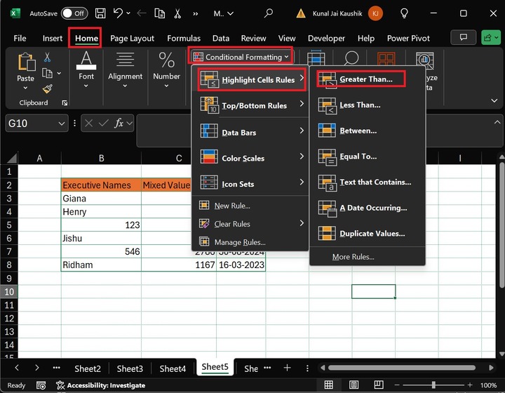
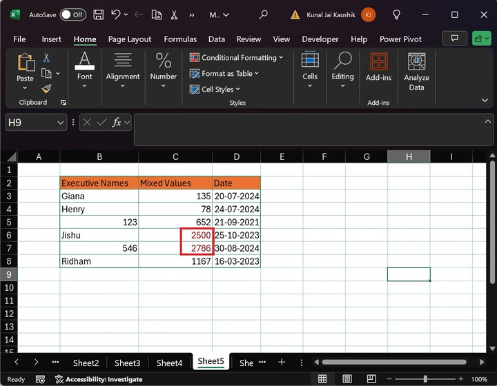
• Highlight cells greater than 2000 with "Red Text" color in the C3: C8 cell range.
• Highlight cell values less than 100 with "Light Red Fill with Dark Red Text color" in the C3:C8 range.
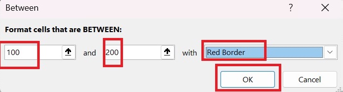
• Highlight cell values reside between 1200 and 1300 with a "Red Border" color in the C3: C8 cell range.
• Highlight cell values equal to 1167 with the "Yellow Fill with Dark Yellow Text" color in the C3: C8 cell range.
• Highlight a cell that contains "Jishu" Text with "Green Fill with Dark Green Text" color in the B3: B8 cell range.
• Highlight cells that contain the date of last month with a "Light Red Fill" color in the cell range D3:D8.

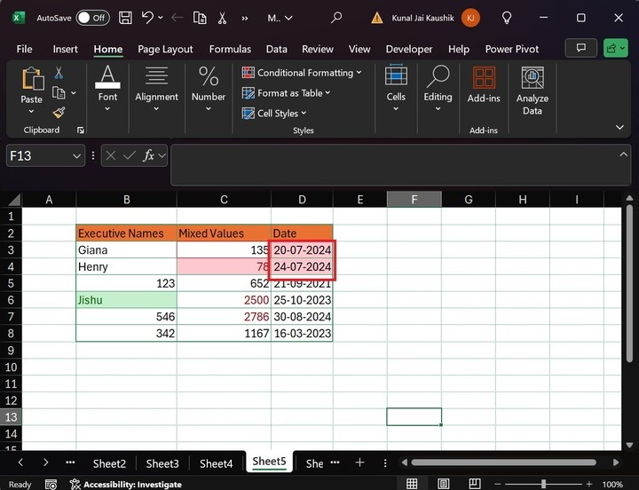
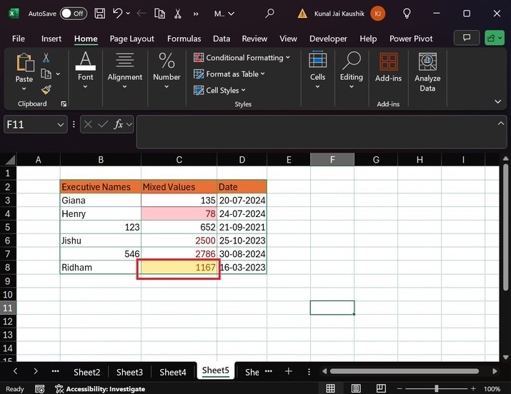
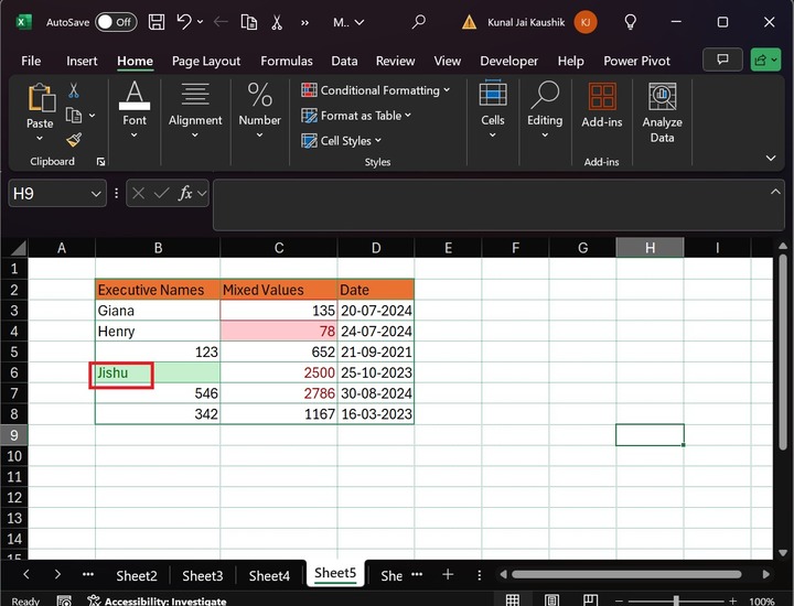
Consider the sample dataset, which comprises three columns titled "Sales Executive", "Mixed Values", and "Dates".

First, select the range C3:C8 and go to the "Home" tab and then switch to the "Conditional Formatting" button, expand the "Highlight Cells Rules" option, and click the "Greater Than…" rule.

After that, write "2000" in the "Format cells that are Greater Than" section and select the "Red Text" color from the drop-down menu. Click the OK button.

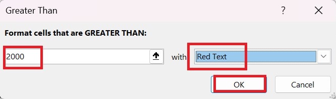
Therefore, cell values exceeded 2000 are highlighted with Red Text color.

After that, select the cell range C3:C8 and choose the Less Than rule from the given list under the "Highlight Cells Rules".

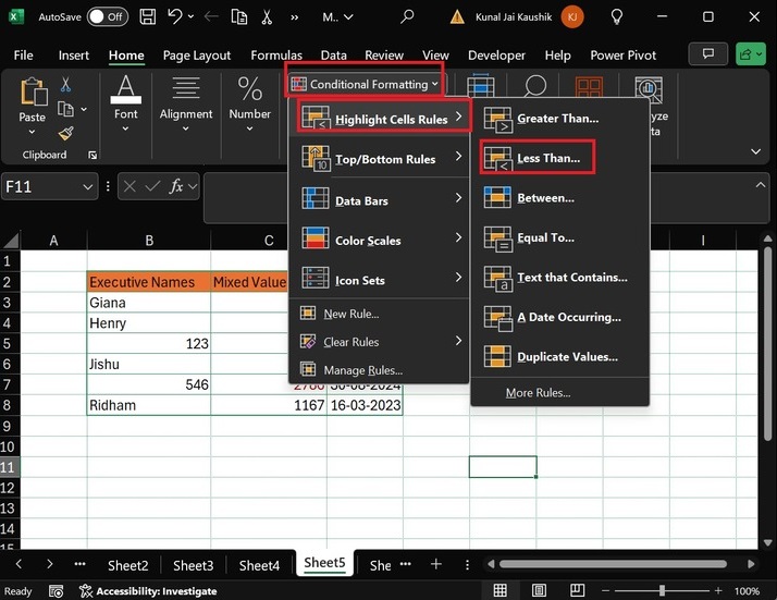
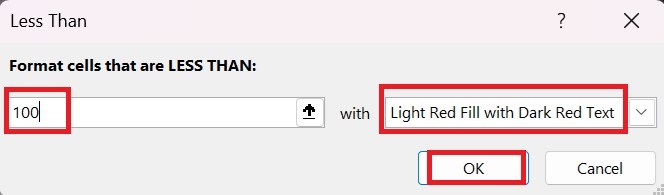
Furthermore, in the "Less Than" dialog box, write "100" in the "Format cells that are LESS THAN:" rule box and select the "Light red Fill with Dark Red Text" color from the given list. Hit the OK button.

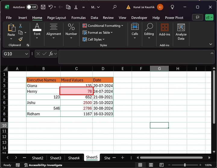
Hence, the cell values that are smaller than 100 are highlighted with the selected color as shown below −

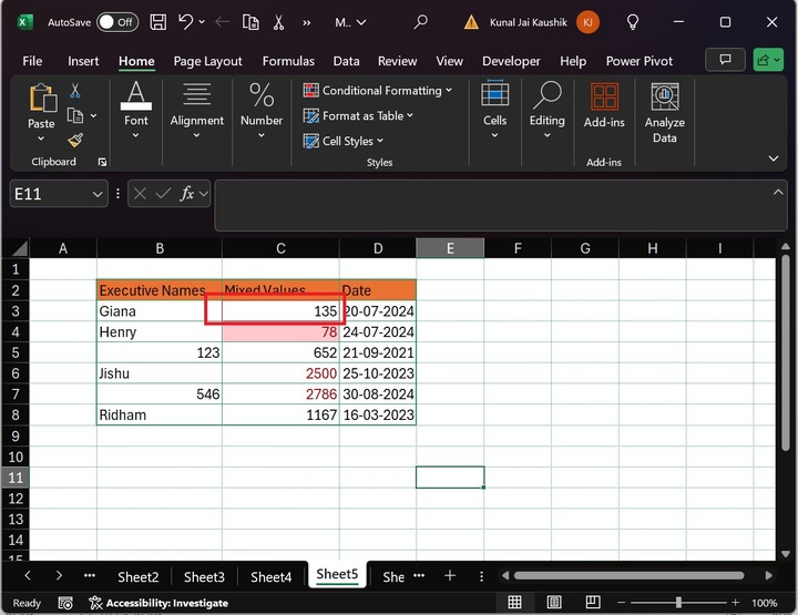
To highlight the numbers that lie between 100 and 200,

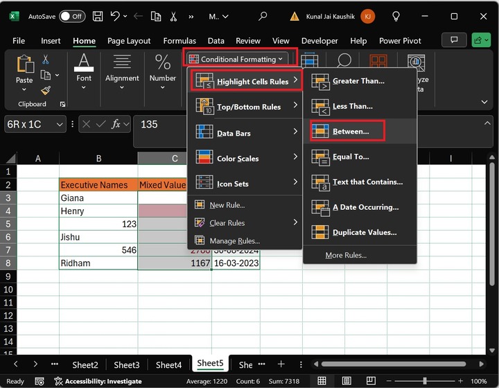
Similarly, select the cell range C3:C8 and expand the "Conditional Formatting" button and click the "Equal To…" rule under the "Highlight Cells Rules" option.

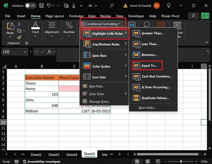
In the Equal To dialog box, write the "1167" in the criteria box in the "Format cells that are EQUAL TO:" section and select the "Yellow Fill with Dark Yellow Text" color from the drop-down menu. And then hit the OK button.

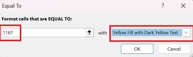
Finally, the 1167 cell value is formatted with Yellow Fill with Dark Yellow Text.

Similarly, select the cell range B3:B8 and click the "Conditional Formatting" button, and choose the "Text that Contains" rule under the "Highlight Cells Rules" option

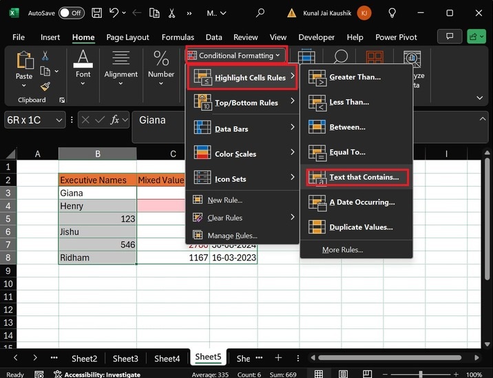
In the "Text That Contains" dialog box, type "Jishu" in the criteria box and select "Green Fill with Dark Green Text," and hit the OK button.

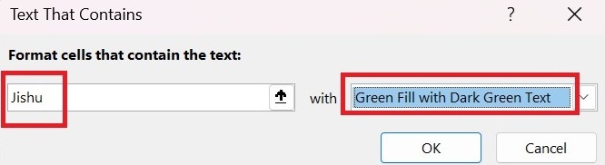
Therefore, cell B6, which contains the "Jishu" is formatted.

Moreover, select the cell range D3:D8 and expand "Conditional Formatting" button, and choose the "A Date Occurring…" rule under the "Highlight Cells Rules" option.

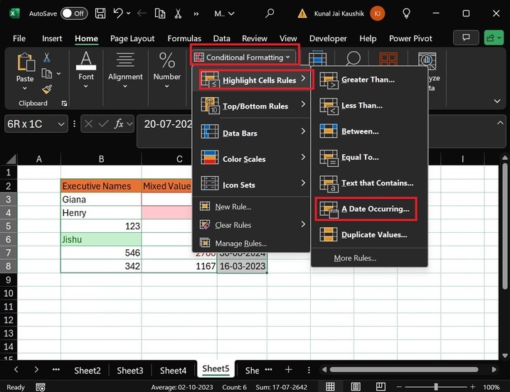
Another dialog box, "A Date Occurring," will appear. In this box, you can select the "Last month" option from the list, choose the "Light Red Fill" color, and click the OK button.

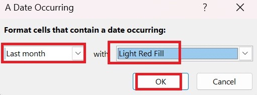
Hence, the last month's dates in the D column are formatted and highlighted with the "Light Red Fill" color.