Excel - Top/Bottom Rules

---

Conditional Formatting Top/Bottom Rule

One of the interesting built-in features of Conditional Formatting is Top/Bottom Rules, which permits you to highlight the top/bottom N values in a specific cell range. For example, the values of the top 5 products, below average and above average student marks, can be highlighted through the top/bottom rules. It works only with quantitative data.

Categories of Top/Bottom Rules

The main categories of the Top/Bottom Rules are given below −

• Top 10 items
• Top 10%
• Bottom 10 Items
• Bottom 10%
• Above Average
• Below Average

The pre-defined color options to highlight a row/column/selected range of the cells are given below −

• Red Border
• Red Text
• Light Red Fill
• Green Fill with Dark Green Text
• Yellow Fill with Dark Yellow Text
• Light Red Fill with Dark Red Text

Lets elaborate on the Conditional Formatting Top/Bottom rules through exciting examples.

Finding Top 10 Quarterly Product Sales Using Top/Bottom Rules

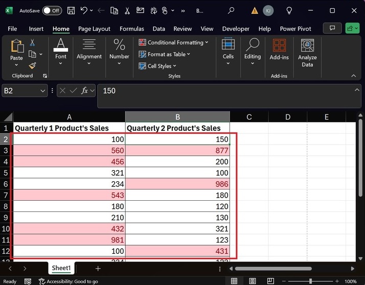
Step 1 − In this example, we will use the Top 10 items rules. Consider the sample dataset, which consists of two columns titled Quarterly 1 Products Sales and Quarterly 2 Products Sales.

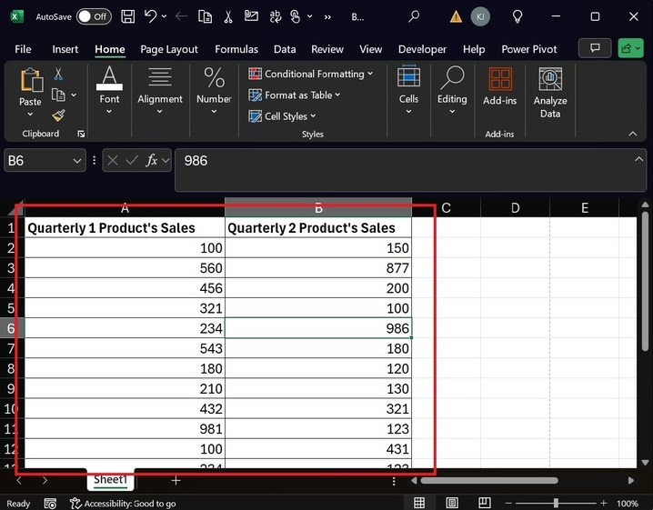
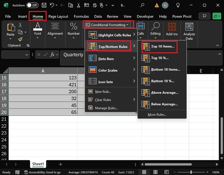
Step 2 − First, select the cell range "A1:B20" and move to the Home tab. Click on the Conditional Formatting button under the Styles group. Expand the Top/Bottom tile and select the "Top 10 Items" from the drop-down menu.

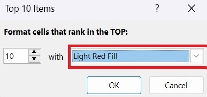
Step 3 − After that, another dialog box, "Top 10 Items," will appear. Select the "Light Red Fill" color from the drop-down list and click OK.

Step 4 − Therefore, the top 10 items in the "Quarterly 1 Product's Sales" column are highlighted with the "Light Red Fill" color.

Similarly, you can highlight the bottom 10 items through the Conditional formattings Top/Bottom rules inbuilt feature.

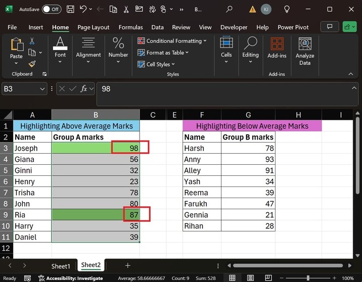
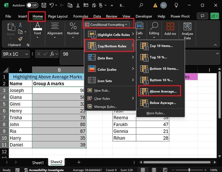
Highlighting above and Below Average Marks for Group A and Group B Students

Step 1 − First, select the cell range B3:B11 and switch to the "Home" tab. Click on "Conditional Formatting" and expand the "Top/Bottom Rules" tile. Then, select the "Above Average" option from the drop-down menu.

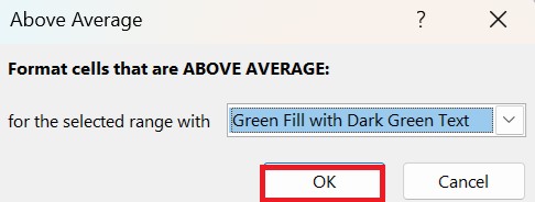
Step 2 − You can select "Green Fill with Dark Green Text" from the list of default formatting colors in the Above Average dialog box. And then hit the OK button.

Step 3 − Therefore, the above-average cell values from the selected range are formatted by highlighting with the "Green Fill with Dark Green Text" color.

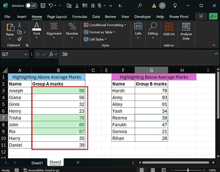
Step 4 − Furthermore, you can select the cell range G3:G10 and proceed with "Home ->Conditional Formatting-> Top/Bottom Rules-> Below Average…" from the drop-down menu.

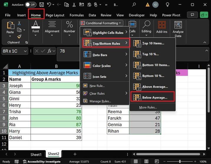
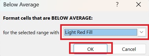
Step 5 − Another dialog box "Below Average" will open. You can choose the "Light Red Fill" color from the drop-down menu and then click the OK button.

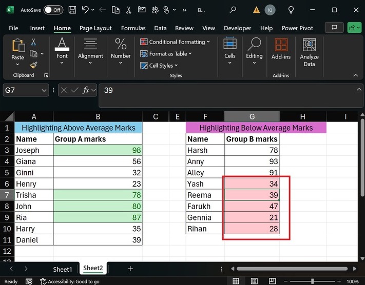
Hence, the below-average marks are highlighted with "Light Red Fill" color as shown below:

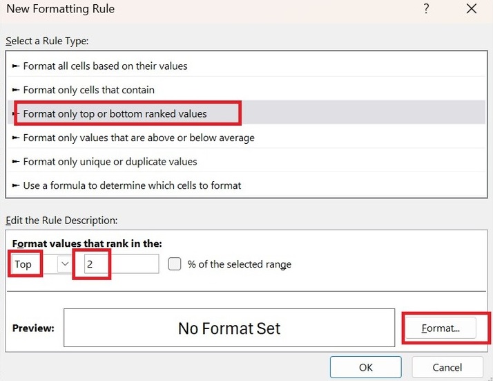
Highlighting Top 2 Values in Excel with Custom Formatting

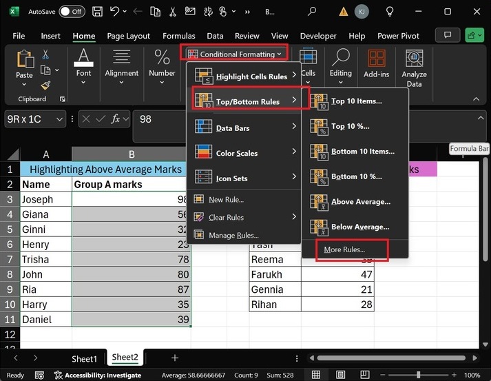
As confined, predefined colors are available in the Top/Bottom Rules. If you wish to customize the colors to highlight the specific column, select the cell range B3:B11 and select the "More Rules" option from the "Top/Bottom Rules" presented in the "Conditional Formatting" tile.

After that, the "New Formatting Rule" dialog box will open. Select the "Format only top or bottom ranked values". In the "Format values that rank in the:" section, select the Top and type "2" in the textbox. Then click on the "Format" button.

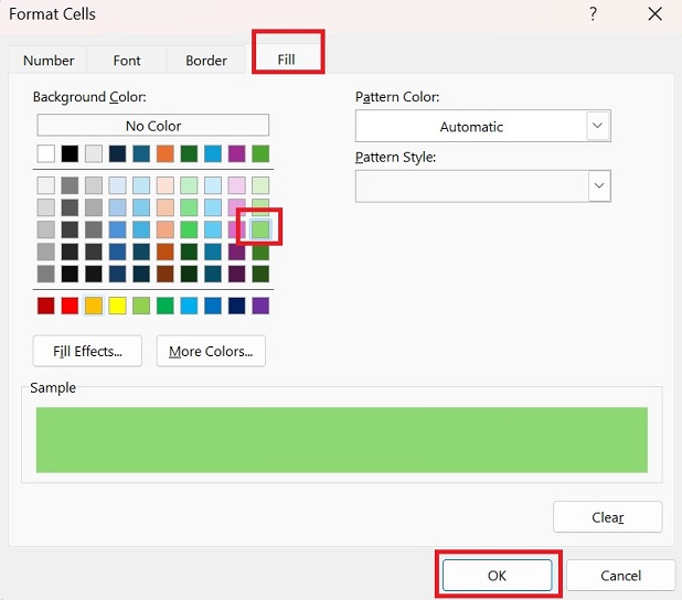
In the "Format Cells" dialog box, go to the "Fill" tab, select the green color, and click the OK button.

Moreover, you can click the OK button in the "New Formatting Rule" window.

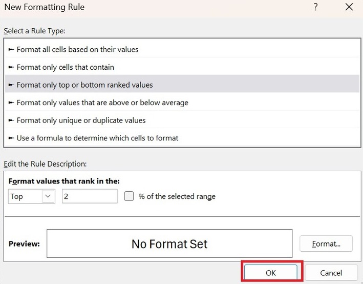
Therefore, the top two marks are highlighted in green.