Excel - Parentheses

---

In Microsoft Excel, the calculation order is changed when you use parentheses ( ) in the expression. The Excel Parentheses have a high priority compared to the other arithmetic operators. For example, in this Excel formula (8*9)+2+3, the multiplication between two numbers inside the parentheses will be computed first, and then the addition part will be computed.

Three variations of the Excel parenthesis are given below −

One Parenthesis − It consists of one pair of parentheses.

For example −

(9/3)+3

Multiple Parentheses − The given formula contains more than one parenthesis.

For example −

(3*2) + (9*8)+(4/2)

Nested Parenthesis − It comprises outer and inner parenthesis.

For example −

 ((9/3)+(4*6)-(18/3))

The inner parenthesis will be evaluated first, then the outer parenthesis will be calculated that is −

((9/3)+(4*6)-(18/3))
= (3+24-6) = 21

How to Add Parentheses in Excel?

The following steps will be taken to add parentheses in Microsoft Excel.

• To add parentheses in the Excel formula, write the = sign and then type the left parenthesis (.
• And then write the expression like 9+8.
• Finally, type the right parentheses) to enclose the expression.
• Therefore, the Excel parentheses in the formula is =(9+8).

Remove Parenthesis in Excel

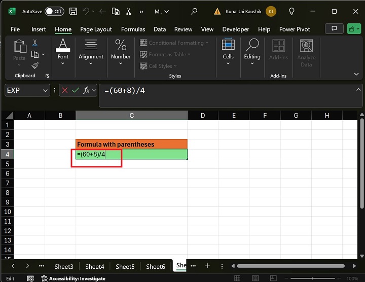
Lets say you have a formula =(60+8)/4.

The following steps will be taken to remove the parentheses in Microsoft Excel −

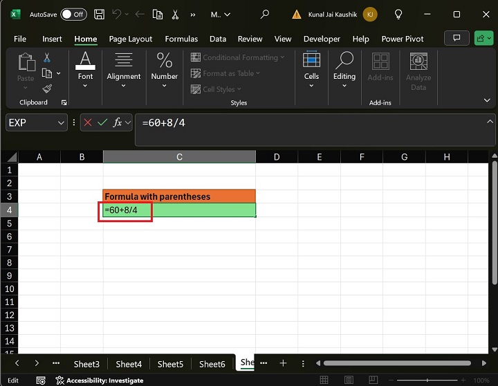
• Use the backspace <- key from the keyboard to remove the left and right parentheses () from the given expression.
• Therefore, the expression with no parentheses is =60+8/4.

Lets see the difference between these two expressions.

Do we get the same result from these two formulas?

=(60+8)/4
=60+8/4

Lets elaborate on these formulas in the Microsoft Excel worksheet. In the C4 cell, enter the formula =(60+8)/4 and press the Enter tab. In this formula, the expression inside the parentheses (60+8) is evaluated first and after that, a division operation will be performed.

Therefore, the result is 17.

After that, enter the formula "=60+8/4" with no parentheses and press the Enter tab. In this expression, the division operation is performed first, and the addition calculation will be calculated.

Therefore, the result is 62.

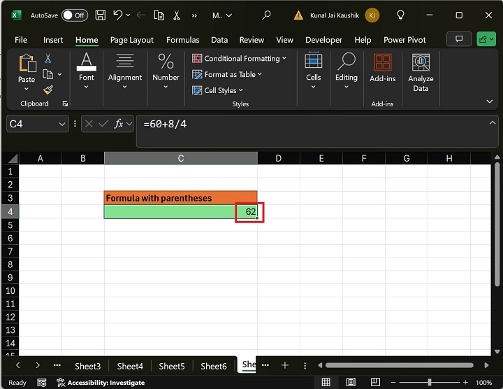
The results of expressions with parenthesis and no parentheses are different.

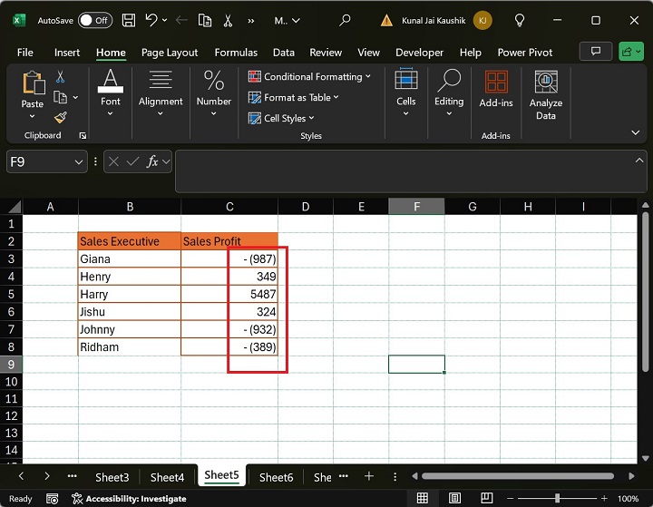
Put Parentheses in Excel for Negative Numbers

Consider the Excel worksheet where the Sales executive's name and Sales profits are specified in the two columns.

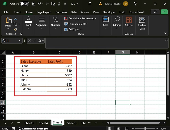
Step 1 − Select the cell range C3:C8 and press the "ctrl+1" key shortcut to open the Format Cells dialog box.

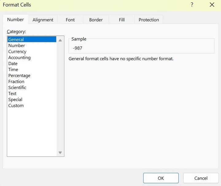
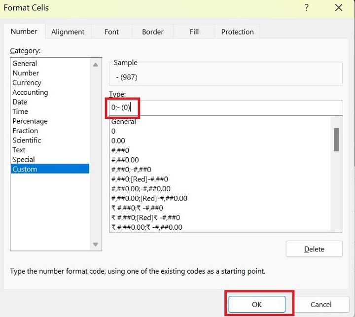
Step 2 − In the Format Cells dialog box, go to the Number tab and select the Custom category, write "0;- (0)" in the Type: box, and click the OK button.

Therefore, negative numbers in parenthesis are showcased in the screenshot below.