Graph Coloring in Discrete Mathematics

---

---

Graph Coloring is an interesting area in Graph Theory that deals with how to efficiently assign colors to vertices in a graph under certain constraints. In this chapter, we will cover the basic concepts of graph coloring. We will understand through examples how Graph Coloring is applied in various scenarios.

What is Graph Coloring?

In simple terms, graph coloring is a problem where we assign colors to elements of a graph. The colors can be assigned on vertices or edges. When specific conditions are met, we can color them.

Primarily, graph coloring is focused on the problem where no two adjacent vertices in a graph share the same color. So this is called the "proper coloring". The minimum number of colors needed to achieve this proper coloring is known as the chromatic number of the graph.

Take a look at the following graph.

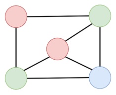
Here, we have 5 vertices and with three colors, we can color the graph. As we need 3 colors as minimum, so the chromatic number for this graph is 3.

The concept of graph coloring came from real-world problems, like map coloring. Consider we are trying to color a map where no two adjacent countries share the same color. When we wish to use as few colors as possible. In graph theory terms, this problem can be rephrased into questions about the chromatic number of a graph. The regions of the map represented by vertices and shared borders by edges.

Vertex Coloring and Chromatic Number

In graph theory, a vertex coloring is the most famous way of coloring. If two vertices are connected by an edge, they are adjacent and cannot share the same color in a proper vertex coloring. The aim is to achieve a proper vertex coloring with the fewest possible colors.

Chromatic Number of a Graph

The chromatic number of a graph G, is denoted as (G). It is the smallest number of colors required to get a proper vertex coloring for the graph. For example, a simple graph with no edges (where no vertices are adjacent) has a chromatic number of 1 because all vertices can be the same color.

Example 1: Chromatic Number of Different Graphs

Consider three graphs and see their coloring idea

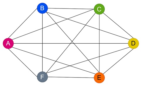
Graph K₆ − In this complete graph of 6 vertices, each vertex is connected to every other vertex. For that a proper vertex coloring, each vertex must have a unique color. So it will have chromatic number of K₆ equal to 6.

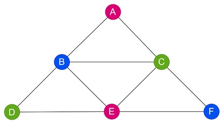
A Triangle Graph − In a triangle (3 vertices each connected to the other two), three colors are needed because each vertex is adjacent to two others. The chromatic number here is 3.

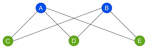
Bipartite Graph K_2,3 − This graph has two sets of vertices, each vertex in one set connected only to vertices in the other set. Here with only two colors (one for each set), we achieve a proper coloring, so the chromatic number is 2.

These examples show that the chromatic number depends on the structure of the graph. So, complete graphs require as many colors as they have vertices, whereas bipartite graphs only need two colors.

The Four-Color Theorem

One of the most famous results in graph theory is the Four Color Theorem. This theorem states that any planar graph (a graph that can be drawn on a plane without crossing edges) has a chromatic number of at most 4. So in practice, any map can be colored using no more than four colors. This is ensuring that no two adjacent regions have the same color.

Here, it has 3 colors but that is less than 4.

Real-World Applications of Graph Coloring

Let us see some practical instances where graph coloring is useful.

Scheduling Problems

In scheduling problems, we can use the idea of graph coloring. It can help determine time slots for events or classes so that conflicts do not arise. Think of a university setting where certain classes cannot be scheduled simultaneously due to shared resources or faculty. By creating a graph with classes as vertices and conflicts as edges, we can assign "colors" (time slots) to each class. We can ensure that no two conflicting classes share the same time.

Example of Classroom Scheduling

Consider a list of classes and their conflicts:

• Class A conflicts with Classes D and I.
• Class B conflicts with D, I, and J.
• Class C conflicts with E, F, and I.

Representing these conflicts as a graph, each class is a vertex, and an edge connects two vertices if their classes conflict. The chromatic number in this graph would represent the minimum number of time slots needed to schedule all classes without any overlapping conflicts.

Frequency Assignment for Radio Stations

Radio stations often use graph coloring to avoid frequency interference with nearby stations. Using graph coloring, we can represent each radio station as a vertex and an edge between two vertices if their frequencies would interfere due to proximity. The chromatic number here would represent the fewest frequencies required to ensure that no nearby stations share the same frequency.

Planar Graphs and Limitations of Chromatic Numbers

As previously mentioned, the chromatic number of planar graphs is constrained by the Four Color Theorem. But, for graphs that are not planar, the chromatic numbers can be higher. The chromatic number can theoretically be unbounded in non-planar graphs. This is making graph coloring a challenge in complex networks.

Example of Non-Planar Graph and Chromatic Number

A complete graph K₅ (5 vertices all connected to each other) has a chromatic number of 5. This graph is not planar, as it cannot be drawn on a plane without crossing edges. Unlike planar graphs, K₅ requires five distinct colors.

Techniques for Estimating Chromatic Numbers

Calculating the exact chromatic number can be challenging. We have certain methods to help to bound:

• Clique Number − A clique in a graph is a subset of vertices that are all adjacent. The largest clique size in a graph, called the clique number. This provides a lower bound for the chromatic number.
• Maximum Degree − The maximum degree Δ(G) of a vertex in a graph gives an upper bound for the chromatic number, with χ(G) ≤ Δ(G) + 1.

Graphs with chromatic numbers equal to their clique numbers are called perfect graphs. Identifying such graphs simplifies the process of finding the chromatic number.

Conclusion

In this chapter, we explained the concept of graph coloring in discrete mathematics. Starting with the basic definitions, we understood how vertex coloring works and what the chromatic number represents.

We looked into specific examples such as complete graphs, triangle graphs, and bipartite graphs to illustrate how chromatic numbers vary with graph structure. We also presented the famous Four Color Theorem and its significance in coloring planar graphs.

We highlighted the practical applications of graph coloring in scheduling and frequency assignment. Furthermore, we understood the techniques for estimating chromatic numbers, including clique number and maximum degree.