Variance and Standard Deviation in Probability Theory

---

---

In Probability Theory, we use the "mean" and "average" to find the center of data, but they don't show how spread out the data is. For that, we need to find the Variance (sometimes called Standard Deviation) that helps us understand how far the values in a data set deviate from the mean.

In this chapter, we will cover the concept of Variance and explain how to calculate Variance using simple examples.

What is Variance?

Variance is a measure of how spread out the data points are from the mean. If all the numbers in a data set are close to the mean, then the variance will be low. If the numbers are spread out far from the mean, the variance will be high. Here the variance gives us an idea of the average squared deviation from the mean.

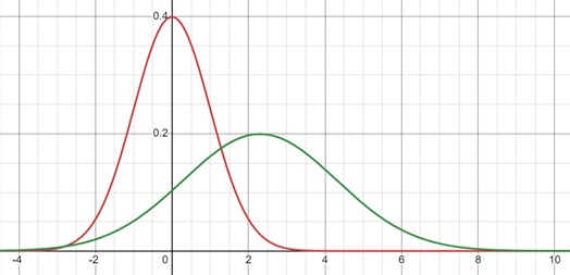
Here, the red curve is with mean 0 and variance 1, and green curve with mean 2.3 and variance 4.

Mathematically, the variance is represented by σ² (for population variance) or s² (for sample variance). We calculate variance by taking the difference between each data point and the mean, squaring those differences (to remove negative values), and then averaging them.

Formula for Variance

For a population variance, the formula is −

$$\mathrm{\sigma^2 \:=\: \frac{1}{N} \sum_{i=1}^{N} (x_i \:-\: \mu)^2}$$

Where −

• N is the number of data points in the population.
• x_i is each individual data point.
• μ is the population mean.

For a sample variance (when we only have a sample of the full population), the formula is slightly different −

$$\mathrm{s^2 \:=\: \frac{1}{n\:-\:1} \sum_{i=1}^{n} (x_i \:-\: \bar{x})^2}$$

Where −

• $\mathrm{{n}}$ is the sample size.
• $\mathrm{\bar{x}}$is the sample mean.
• $\mathrm{x_i}$ is each individual data point.

We divide by n − 1 instead of n for sample variance. This is called Bessel's correction. It adjusts for the fact that a sample may underestimate the true population variance.

Example of Calculating Variance

Let us find the variance for two different data sets. Consider the following data sets −

• Data set 1: −10, 0, 10, 20, 30
• Data set 2: 8, 9, 10, 11, 12

Step 1: Calculate the Mean

First, we calculate the mean for both the data sets −

For data set 1 −

$$\mathrm{\mu \:=\: \frac{-10 \:+\: 0 \:+\: 10 \:+\: 20 \:+\: 30}{5} \:=\: 10}$$

For data set 2 −

$$\mathrm{\mu \:=\: \frac{8 \:+\: 9 \:+\: 10 \:+\: 11 \:+\: 12}{5} \:=\: 10}$$

Both data sets have the same mean, which is 10, but we will see that their spread (variance) is very different.

Step 2: Calculate the Squared Differences

Now, we calculate how far each number in the data sets is from the mean, square those differences, and sum them up.

For data set 1 −

Squared differences $\mathrm{= \:(-10 \:-\: 10)^2 \:+\: (0 \:-\: 10)^2 \:+\: (10 \:-\: 10)^2 \:+\: (20 \:-\: 10)^2 \:+\: (30 \:-\: 10)^2}$

$$\mathrm{=\: (-20)^2 \:+\: (-10)^2 \:+\: (0)^2 \:+\: (10)^2 \:+\: (20)^2}$$

$$\mathrm{=\: 400 \:+\: 100 \:+\: 0 \:+\: 100 \:+\: 400 \:=\: 1000}$$

For data set 2 −

Squared differences $\mathrm{= (8 - 10)^2 + (9 - 10)^2 + (10 - 10)^2 + (11 - 10)^2 + (12 - 10)^2}$

$$\mathrm{=\: (-2)^2 \:+\: (-1)^2 \:+\: (0)^2 \:+\: (1)^2 \:+\: (2)^2}$$

$$\mathrm{=\: 4 \:+\: 1 \:+\: 0 \:+\: 1 \:+\: 4 \:=\: 10}$$

Step 3: Calculate the Variance

Now we divide by the number of data points (for population variance) to find the variance.

For data set 1 −

$$\mathrm{\sigma^2 \:=\: \frac{1000}{5} \:=\: 200}$$

For data set 2 −

$$\mathrm{\sigma^2 \:=\: \frac{10}{5} \:=\: 2}$$

So, the variance of data set 1 is 200, while the variance of data set 2 is only 2. This shows that data set 1 is much more spread out from the mean than data set 2.

What is Standard Deviation?

Variance gives us an idea of the spread of data. It is measured in squared units (like meters squared if the data is in meters). We can feel a bit abstract. To bring it back to the original units, we take the square root of the variance, which is known as standard deviation.

Standard deviation is represented by σ for population data and s for sample data. It is simply the square root of the variance −

$$\mathrm{\sigma \:=\: \sqrt{\sigma^2}}$$

The standard deviation gives us a more intuitive sense of how spread out the data. It is by providing the typical distance from the mean in the original units of the data.

Example of Calculating Standard Deviation

Let us see the example again and calculate the standard deviation for the two data sets.

For data set 1 −

$$\mathrm{\sigma \:=\: 200 \:\approx\: 14.14}$$

For data set 2 −

$$\mathrm{\sigma \:=\: 2 \:\approx\: 1.41}$$

So, the standard deviation for data set 1 is much larger than that of data set 2, confirming that data set 1 is more spread out.

Interpretation of Standard Deviation

The standard deviation is much useful tool. This gives us a clearer idea of how spread out the data is. A small standard deviation means that the data points are close to the mean, and large standard deviation means the data points are spread out.

For instance, in our example −

• Data set 2 has a standard deviation of 1.41, meaning the numbers in that set are typically within 1.41 units of the mean (which was 10).
• Data set 1, however, has a standard deviation of 14.14, meaning its numbers are usually much farther from the mean.

Why Do We Need to Square the Differences?

We might think why we square the differences when calculating the variance. The reason is as given below −

• To remove negative values − Simply subtracting the mean from each data point would result in negative values for numbers smaller than the mean. By squaring the differences, we will get all the values are positive.
• To emphasize larger deviations − Squaring larger differences makes them stand out more. For example, if a data point is far from the mean, then its squared difference will be much longer. It reflects its impact on the overall variance.

Range: A Simple Measure of Spread

Another way to measure the spread of data is the range. This is the difference between the largest and smallest values in the data set. The range is easy to calculate. It does not give a full picture of how the data is spread out.

For example, when data sets might have the same range but very different standard deviations if the values are clustered differently.

Example of Range

For data set 1 −

Range = 30 (10) = 40

For data set 2 −

Range = 12 8 = 4

Clearly, the range shows that data set 1 is more spread out, but it does not capture how the numbers are distributed. Variance and standard deviation give us a deeper understanding.

Conclusion

In this chapter, we explained how Variance and Standard Deviation help us find the spread of a data set. Variance gives us the average of the squared differences from the mean.

Standard deviation gives us a more intuitive way of dispersion by taking the square root of the variance. We explained how Variance and Standard Deviation give us valuable insight on how the data is distributed.