Distribution Functions in Probability Theory

---

---

Distribution functions help us understand and predict the likelihood of different outcomes. Distribution functions describe how probabilities are assigned to different possible outcomes of a random variable. They help us make sense of both discrete and continuous data.

Read this chapter to learn the various types of distribution functions, including Probability Mass Functions (PMFs), Probability Density Functions (PDFs), and Cumulative Distribution Functions (CDFs).

What is a Distribution Function?

A distribution function in probability theory states how probability is spread across possible outcomes for a random variable. It can take the form of −

• A discrete random variable, where the outcomes are distinct and separate (like rolling a die).
• A continuous random variable, where the outcomes can take on any value within a range (like measuring height).

Different types of distribution functions are used depending on whether the random variable is discrete or continuous.

Discrete Random Variables: Probability Mass Function (PMF)

For discrete random variables, we generally use the idea of Probability Mass Function (PMF). This PMF tells us the probability that a random variable takes on a specific value.

Example of Rolling a Die

A simple example of a discrete random variable is rolling a six-sided die. There are six possible outcomes: 1, 2, 3, 4, 5, and 6. Assuming the die is fair and there is no biases. The probability of landing on any one number is 1/6, or about 0.167.

So, the PMF for rolling a die would look something like this −

$$\mathrm{P(X \:=\: x) \:=\: \begin{cases} \frac{1}{6},\: & \text{if } x \:=\: 1,\: 2,\: 3,\: 4,\: 5,\: 6 \\\\ 0,\: & \text{otherwise} \end{cases}}$$

In this case, X is our random variable (the number rolled on the die), and the PMF assigns a probability of 1/6 to each outcome.

Cumulative Distribution Function for Discrete Variables

Then the next function is the CDF. For discrete variables, we can also create a Cumulative Distribution Function (CDF). This CDF shows us the probability that a random variable takes on a value less than or equal to a certain number.

If we continuing with the die example, the CDF would describe the probability of rolling a number less than or equal to each possible outcome. If we are interested in the probability of rolling a 4 or less, we would add up the probabilities of rolling a 1, 2, 3, or 4:

$$\mathrm{P(X \:\leq\: 4) \:=\: P(X \:=\: 1) \:+\: P(X \:=\: 2) \:+\: P(X \:=\: 3) \:+\: P(X \:=\: 4) \:=\: \frac{4}{6} \:=\: 0.667}$$

So, the CDF at 4 would be 0.667. And as expected, by the time we reach 6, the CDF should equal 1, because the probability of rolling a number 6 or less is 100%.

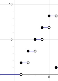
This figure shows CDF for 6 rolls with 100%.

Continuous Random Variables: Probability Density Function

For continuous random variables, we use a Probability Density Function (PDF) instead of a PMF. The PDF describes the likelihood of the random variable falling within a certain range. Not taking on specific values.

Example: Height Distribution

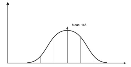
Imagine we are looking at the heights of women, which might be distributed in a bell-shaped curve (a normal distribution). The heights are a continuous variable since someone can be 165.4 cm tall, or 165.387 cm tall, and so on. The PDF gives us a picture of how likely different heights are. It does not give exact probabilities for specific values.

For example, the probability that someone is exactly 165 cm tall is essentially zero, because there are infinitely many possible heights in the range. However, we can use the PDF to calculate the probability of someone being between, say, 160 cm and 170 cm.

The graph of the PDF for height might peak around the mean (165 cm, for example) and taper off as we get farther from the average height. The higher the peak, the more likely someone is to be around that height.

Cumulative Distribution Function for Continuous Variables

Like the discrete variables, we can construct a Cumulative Distribution Function (CDF) for continuous variables as well. The CDF for a continuous variable shows the probability that the variable takes on a value less than or equal to a certain number.

For instance, if we are finding the probability that a woman's height is less than or equal to 165 cm, we can get the CDF. In this case, it might tell us that the probability is 0.5, meaning 50% of women are shorter than or equal to 165 cm.

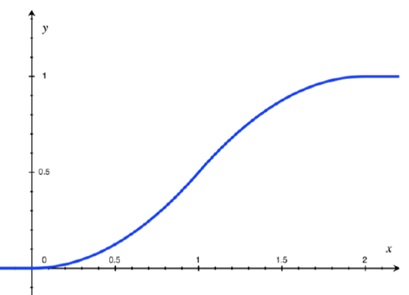
The CDF for continuous variables looks like an S-shaped curve. It starts at 0 (no probability accumulated at the beginning), gradually increases as we move along the distribution, and eventually reaches 1 (meaning all the probability is accounted for) as we cover the entire range of possible values.

Understanding the Relationship Between PDF and CDF

We must understand how the PDF and CDF are related. The PDF is like the "instantaneous" rate of change of the CDF. We can also say that the gradient or slope of the CDF at any point is the value of the PDF at that point.

If the CDF has a steep slope at a certain point, which means the PDF has a high value there. Which indicates a higher probability density around that value. For example, in our height distribution example, the PDF will peak around the average height. That corresponds to the steepest part of the CDF.

Mathematically, if F(x) is the CDF, then the PDF f(x) is the derivative of the CDF −

$$\mathrm{f(x) \:=\: \frac{d}{dx} F(x)}$$

Conversely, if we integrate the PDF from negative infinity up to a certain value x, we recover the CDF −

$$\mathrm{F(x) \:=\: \int_{-\infty}^{x}\: f(t) \: dt}$$

This shows that the CDF and PDF are two sides of the same coin. They are deeply connected.

CDF and PDF in Action

Let us see the same example again. The PDF shows where the density of heights is concentrated. So the closer someones height is to the average, the higher the PDF. On the other hand, the CDF shows that what percentage of the population is shorter than a given height.

Finding the Probability for a Range of Heights

Suppose we want to find the probability that a womans height is between 160 cm and 170 cm. We would use the CDF to calculate this by finding the CDF value at 170 cm and subtracting the CDF value at 160 cm −

$$\mathrm{P(160 \leq X \leq 170) = F(170) - F(160)}$$

This gives the probability that the height is within that range.

Discrete vs Continuous: The Difference

To summarize the key differences between discrete and continuous random variables, we can conclude −

• PMF (Probability Mass Function) is used for discrete random variables. It gives probabilities to specific outcomes, like rolling a 1 or 2 on a die.
• PDF (Probability Density Function) is used for continuous random variables. It gives a "density" of probability over a range, not exact values.

Both discrete and continuous random variables have Cumulative Distribution Functions (CDFs), which gives us the probability that a variable is less than or equal to a given value.

Conclusion

Distribution Functions form the backbone of Probability Theory. We explained the Probability Mass Function (PMF) for discrete random variables, for example rolling a die; and the Probability Density Function (PDF) for continuous variables, for example, measuring height. We also covered the Cumulative Distribution Function (CDF) and how it works for both discrete and continuous variables.