Assemble Images with Simple Image Stitching

Image stitching is a fundamental task in computer vision and image processing, allowing us to seamlessly combine multiple images into a single, larger composite image. This process is particularly useful when we assume rigid body motions, such as translations and rotations, between the images.

In this tutorial, we will explore the step-by-step process of assembling images under the assumption of rigid body motions. We'll cover key aspects of image stitching, including the detection of interest points, matching these points, estimating transformations, and the final step of combining the images to create a single, stitched result.

Example

The following example demonstrates how to perform image registration by matching features in a set of images and applying affine transformations to align them with a reference image.

from matplotlib import pyplot as plt
import numpy as np
from skimage import data, util, transform, feature, measure, filters, metrics

def match_image_locations(image0, image1, reference_coords, candidate_coords, patch_radius=5, gaussian_sigma=3):
    
   y, x = np.mgrid[-patch_radius:patch_radius + 1, -patch_radius:patch_radius + 1]
   weights = np.exp(-0.5 * (x ** 2 + y ** 2) / gaussian_sigma ** 2)
   weights /= 2 * np.pi * gaussian_sigma * gaussian_sigma
   
   matched_coords = []
   for r0, c0 in reference_coords:
      patch0 = image0[r0 - patch_radius:r0 + patch_radius + 1, c0 - patch_radius:c0 + patch_radius + 1]
      candidate_patches = [image1[r1 - patch_radius:r1 + patch_radius + 1, c1 - patch_radius:c1 + patch_radius + 1] for r1, c1 in candidate_coords]
      ssd_list = [np.sum(weights * (patch0 - candidate_patch) ** 2) for candidate_patch in candidate_patches]
      matched_coords.append(candidate_coords[np.argmin(ssd_list)])
   
   return np.array(matched_coords)

# Data Generation
reference_image = data.moon()

tilt_angles = [0, 5, 6, -2, 3, -4]
center_coordinates = [(0, 0), (10, 10), (5, 12), (11, 21), (21, 17), (43, 15)]

image_list = [transform.rotate(reference_image, angle=a, center=c)[40:240, 50:350] for a, c in zip(tilt_angles, center_coordinates)]
reference_image_copy = image_list[0].copy()

image_list = [util.random_noise(filters.gaussian(image, 1.1), var=5e-4, rng=seed) for seed, image in enumerate(image_list)]
reference_psnr = metrics.peak_signal_noise_ratio(reference_image_copy, image_list[0])

# Image Registration
min_distance = 5
corners_list = [feature.corner_peaks(feature.corner_harris(image), threshold_rel=0.001, min_distance=min_distance) for image in image_list]

# Use the corners detected in the first image as reference points
reference_image = image_list[0]
reference_coords = corners_list[0]
matched_corners = [match_image_locations(reference_image, image, reference_coords, candidate_coords, min_distance) for image, candidate_coords in zip(image_list, corners_list)]

# Estimate robust relative affine transformations using RANSAC
source = np.array(reference_coords)
transformations = [measure.ransac((destination, source), transform.EuclideanTransform, min_samples=3, residual_threshold=2, max_trials=100)[0].params for destination in matched_corners]

# Display the Results
fig, ax_list = plt.subplots(6, 2, figsize=(6, 9), sharex=True, sharey=True)
for index, (image, transform_params, (axis0, axis1)) in enumerate(zip(image_list, transformations, ax_list)):
   axis0.imshow(image, cmap="gray", vmin=0, vmax=1)
   axis1.imshow(transform.warp(image, transform_params), cmap="gray", vmin=0, vmax=1)
   
   if index == 0:
      axis0.set_title("Tilted Images")
      axis0.set_ylabel(f"Reference Image\n(PSNR={reference_psnr:.2f})")
      axis1.set_title("Registered Images")
   
   axis0.set(xticklabels=[], yticklabels=[], xticks=[], yticks=[])
   axis1.set_axis_off()

fig.tight_layout()
plt.show()

Output

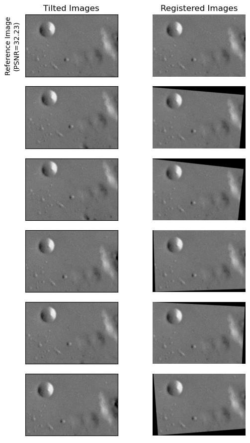
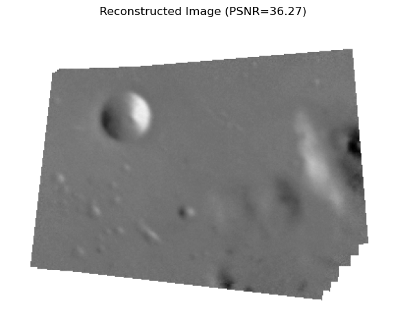
Image assembling

To create a composite image, we position the registered images relative to the reference image within a global domain. We achieve this by defining a global transformation, which essentially relocates the reference image within this global domain through a straightforward translation.

Example

In this continuation of the previous example, we define the margin and output shape for the global transformation. We then apply this transformation to all images in the image_list, creating a global_image_list. A mask is used to identify areas with NaN values, and these areas are set to 1 to avoid NaN artifacts. Finally, a composite image is created by averaging the global image list, and its Peak Signal-to-Noise Ratio (PSNR) is calculated and displayed.

# Define the margin and output shape for global transformation
margin = 50
height, width = image_list[0].shape
output_shape = height + 2 * margin, width + 2 * margin

# Initialize the global transformation matrix as an identity matrix
global_transform = np.eye(3)
global_transform[:2, 2] = -margin, -margin

# Apply global transformation to all images and create a global image list
global_image_list = [transform.warp(image, transformation.dot(global_transform),
      output_shape=output_shape,
      mode="constant", cval=np.nan)
   for image, transformation in zip(image_list, transformations)]

# Create a mask to identify areas with NaN values
all_nan_mask = np.all([np.isnan(image) for image in global_image_list], axis=0)
global_image_list[0][all_nan_mask] = 1.

# Create a composite image by averaging the global image list
composite_image = np.nanmean(global_image_list, axis=0)
composite_psnr = metrics.peak_signal_noise_ratio(reference_image_copy,
   composite_image[margin:margin + height,
      margin:margin + width])

# Display the reconstructed composite image
figure, axis = plt.subplots(1, 1)

axis.imshow(composite_image, cmap="gray", vmin=0, vmax=1)
axis.set_axis_off()
axis.set_title(f"Reconstructed Image (PSNR={composite_psnr:.2f})")
figure.tight_layout()

plt.show()

Output