Scikit Image - Warping an image

Quiz

Image warping refers to the process of transforming an image from its original coordinate space to a new coordinate space, typically to achieve geometric transformations. The goal is to remap the pixels of the input image to new positions in the output image, according to a specified transformation function. This process is commonly used in various image-processing tasks to achieve effects like rotation, scaling, and perspective transformations.

In scikit-image, The skimage.transform.warp(), skimage.transform.warp_coords() and skimage.transform.warp_polar() functions are used to perform image warping tasking in Pythons scikit-image library.

Using the skimage.transform.warp() function

The warp() function in scikit-image is used to warp an image based on a given coordinate transformation.

Syntax

Following is the syntax of this function −

skimage.transform.warp(image, inverse_map, map_args=None, output_shape=None, order=None, mode='constant', cval=0.0, clip=True, preserve_range=False)

Parameters

image: The input image to be warped, represented as a NumPy array.
inverse_map: The coordinate transformation that maps coordinates in the output image to their corresponding coordinates in the input image. This can be specified in different ways, depending on the dimensionality of the input image.
map_args (optional): Keyword arguments passed to the inverse_map.
output_shape (optional): The desired shape of the output image. By default, it preserves the shape of the input image.
order (int, optional): The order of spline interpolation used during the rotation. The default value is 0 if the image.dtype is bool and 1 otherwise. The order must be in the range 0-5.
order (optional): The order of interpolation used during warping.
mode (optional): Determines how points outside the boundaries of the input image are filled. It can take values like 'constant', 'edge', 'symmetric', 'reflect', or 'wrap'.
cval (optional): The value used for points outside the image when mode is set to 'constant.
clip (optional): Specifies whether to clip the output to the range of values of the input image. It is enabled by default to avoid values outside the input range.
preserve_range (optional): Specifies whether to keep the original range of values. If set to False, the input image is converted according to the conventions of img_as_float.

Return Value

It returns the warped output image, a double NumPy array representing the warped input image.

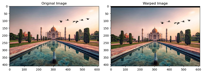
Example

Here is an example of using the skimage.transform.warp() function to warp an image using a geometric transform (fast).

from skimage.transform import SimilarityTransform, warp
from skimage import io
import matplotlib.pyplot as plt

# Load the input image 
image = io.imread('Images/Tajmahal.jpg')

# Define the geometric transform (translation by 10 pixels upwards)
tform = SimilarityTransform(translation=(0, -10))

# Apply the warp using the defined transform
warped = warp(image, tform)

# Display the original and  warped mages side by side
fig, axes = plt.subplots(1, 2, figsize=(10, 5))
axes[0].imshow(image)
axes[0].set_title('Original Image')

axes[1].imshow(warped)
axes[1].set_title('Warped Image')

# Show the plot
plt.tight_layout()
plt.show()

Output

On executing the above program, you will get the following output −

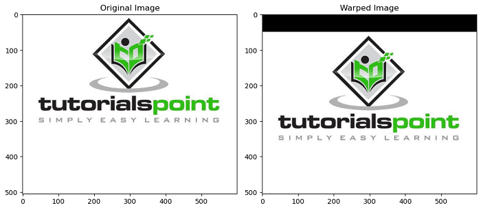
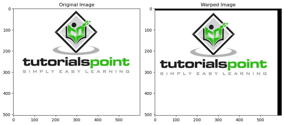
Example

The following example demonstrates how to warp an image using a custom callable (slow) using the skimage.transform.warp() function.

from skimage.transform import SimilarityTransform, warp
from skimage import io
import matplotlib.pyplot as plt

def shift_down(xy):
    xy[:, 1] -= 50
    return xy

# Load the input image 
image = io.imread('Images/logo.jpg')

# Apply the warp using the defined transform
warped = warp(image, shift_down)

# Display the original and  warped mages side by side
fig, axes = plt.subplots(1, 2, figsize=(10, 5))
axes[0].imshow(image)
axes[0].set_title('Original Image')

axes[1].imshow(warped)
axes[1].set_title('Warped Image')

# Show the plot
plt.tight_layout()
plt.show()

Output

On executing the above program, you will get the following output −

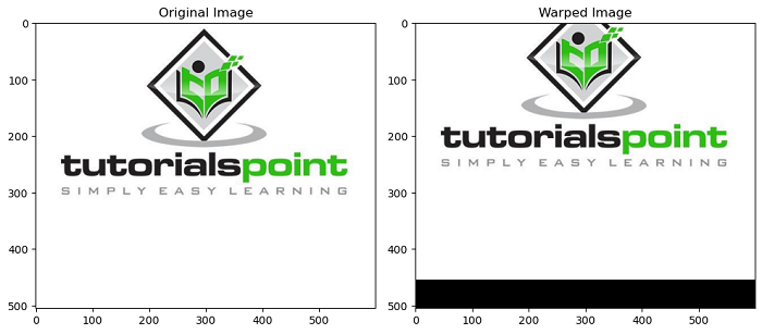
Example

In this example, we will use a 2D transformation matrix to represent a translation of 50 pixels in the vertical direction (upward).

from skimage.transform import SimilarityTransform, warp
from skimage import io
import matplotlib.pyplot as plt
import numpy as np

# Load the input image 
image = io.imread('Images/logo.jpg')

# Define a 2D transformation matrix for translation (50 pixels upward)
matrix = np.array([[1, 0, 0], [0, 1, 50], [0, 0, 1]])

# Apply the warp using the transformation matrix
warped = warp(image, matrix)

# Display the original and  warped mages side by side
fig, axes = plt.subplots(1, 2, figsize=(10, 5))
axes[0].imshow(image)
axes[0].set_title('Original Image')

axes[1].imshow(warped)
axes[1].set_title('Warped Image')

# Show the plot
plt.tight_layout()
plt.show()

Output

On executing the above program, you will get the following output −

Using the skimage.transform.warp_coords() function

The warp_coords function is used to build the source coordinates for the output of a 2-D image warp. This function is provided separately from warp() to give users additional flexibility, allowing them to reuse specific coordinate mappings or use specific data types during the image-warping process. It returns the coordinates that can be passed to scipy.ndimage.map_coordinates to obtain the desired warped image.

Syntax

Following is the syntax of this function −

skimage.transform.warp_coords(coord_map, shape, dtype=<class 'numpy.float64'>)

Parameters

coord_map: A callable (e.g., a GeometricTransform.inverse) that takes the output coordinates as input and returns the corresponding input coordinates. The input and output coordinates are both represented as a (P, 2) array, where P is the number of coordinates, and each element is a (row, col) pair.
shape: A tuple representing the shape of the output image (rows, cols[, bands]).
dtype: The data type for the return value. Sane choices are float32 or float64.

Return Value

It returns an array representing the coordinates for scipy.ndimage.map_coordinates. The shape of the coordinates is (ndim, rows, cols[, bands]), and the data type is determined by the dtype parameter.

Example

Here is an example to produce a coordinate map that shifts an image up and to the right using the skimage.transform.warp_coords() function.

from skimage.transform import warp_coords
from skimage import io
from scipy.ndimage import map_coordinates
import matplotlib.pyplot as plt
import numpy as np

def shift_up10_left20(xy):
    return xy - np.array([-20, 10])[None, :]

# Load the input image 
image = io.imread('Images/logo.jpg')

# Get the coordinates for the image warp using the coordinate map
coords = warp_coords(shift_up10_left20, image.shape)

# Perform the image warp using scipy.ndimage.map_coordinates
warped_image = map_coordinates(image, coords)

# Display the original and  warped mages side by side
fig, axes = plt.subplots(1, 2, figsize=(10, 5))
axes[0].imshow(image)
axes[0].set_title('Original Image')

axes[1].imshow(warped_image)
axes[1].set_title('Warped Image')

# Show the plot
plt.tight_layout()
plt.show()

Output

On executing the above program, you will get the following output −

Using the skimage.transform.warp_polar function

The warp_polar() function is used to remap an input image to polar or log-polar coordinate space.

Syntax

Following is the syntax of this function −

skimage.transform.warp_polar(image, center=None, *, radius=None, output_shape=None, scaling='linear', channel_axis=None, **kwargs)

Parameters

image: The input image to be warped. It should be a 2-D array for grayscale images or a 3-D array for color images (channel_axis parameter should be specified).
center: A tuple representing the center point in the image, which serves as the origin in Cartesian space for the polar transformation. If not provided, the center is assumed to be the center point of the image.
radius: The radius of the circle that bounds the area to be transformed.
output_shape: A tuple representing the shape of the output warped image in polar coordinates.
scaling: Specify whether the image warp is polar ('linear') or log-polar ('log'). The default is 'linear'.
channel_axis: An integer or None, indicating the axis of the array that corresponds to channels. If None, the image is assumed to be a grayscale image. If specified, the function accepts 3-D arrays (for color images) with the specified axis as the channel axis.

Return Value

It returns a ndarray representing the polar or log-polar warped image.

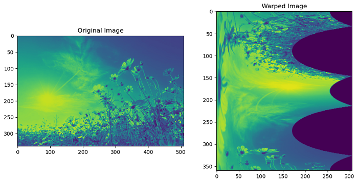
Example

The following example demonstrates how to perform a basic polar warp on a grayscale image using the warp_polar() function.

from skimage import io
from skimage.transform import warp_polar
import matplotlib.pyplot as plt

# Load the input image as gray-scale image
image = io.imread('Images/flowers.jpg', as_gray=True)

# Perform a basic polar warp on the grayscale image
warped = warp_polar(image)

# Display the original and  warped mages side by side
fig, axes = plt.subplots(1, 2, figsize=(10, 5))
axes[0].imshow(image)
axes[0].set_title('Original Image')

axes[1].imshow(warped)
axes[1].set_title('Warped Image')

# Show the plot
plt.tight_layout()
plt.show()

Output

On executing the above program, you will get the following output −

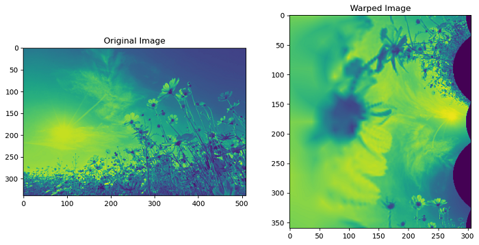
Example

The following example demonstrates how to perform the log-polar warp on a grayscale image using the warp_polar() function.

from skimage import io
from skimage.transform import warp_polar
import matplotlib.pyplot as plt

# Load the input image as gray-scale image
image = io.imread('Images/flowers.jpg', as_gray=True)

# Perform the log-polar warp on the grayscale image
warped = warp_polar(image, scaling='log')

# Display the original and  warped mages side by side
fig, axes = plt.subplots(1, 2, figsize=(10, 5))
axes[0].imshow(image)
axes[0].set_title('Original Image')

axes[1].imshow(warped)
axes[1].set_title('Warped Image')

# Show the plot
plt.tight_layout()
plt.show()

Output

On executing the above program, you will get the following output −

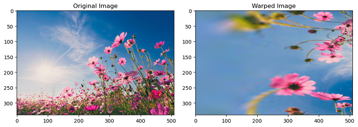
Example

The following example demonstrates how to perform a log-polar warp on the color image while specifying the center, radius, and output shape using the warp_polar() function.

from skimage import io
from skimage.transform import warp_polar
import matplotlib.pyplot as plt

# Load the input image as gray-scale image
image = io.imread('Images/flowers.jpg')

# Perform a log-polar warp on the color image while specifying the center, radius, and output shape
warped = warp_polar(image, center=(150, 300), radius=100, output_shape=image.shape, scaling='log', channel_axis=-1)

# Display the original and  warped mages side by side
fig, axes = plt.subplots(1, 2, figsize=(10, 5))
axes[0].imshow(image)
axes[0].set_title('Original Image')

axes[1].imshow(warped)
axes[1].set_title('Warped Image')

# Show the plot
plt.tight_layout()
plt.show()

Output

On executing the above program, you will get the following output −

Print Page