Scikit Image - Convex Hull

---

---

A convex hull is referred to as the smallest convex polygon or shape that completely encloses a given set of points, it is a fundamental concept in image processing. This concept is often used in various applications such as image segmentation, pattern recognition, and computer vision to simplify and understand the structure of complex shapes within an image.

The scikit-image library provides the convex_hull_image() and convex_hull_object() functions in the skimage.morphology model to perform the morphological operations on the binary image.

Using the skimage.morphology.convex_hull_image() function

The morphology.convex_hull_image() function is used to compute the convex hull of a binary image. The convex hull is the smallest convex polygon that surrounds all the white pixels in the input binary image.

Syntax

Following is the syntax of this function −

skimage.morphology.convex_hull_image(image, offset_coordinates=True, tolerance=1e-10, include_borders=True)

Parameters

• image: This is the input binary image for which you want to compute the convex hull. The function automatically converts this array to a boolean type before processing.
• offset_coordinates (optional): If set to True, it means that each pixel will be treated as having some extent, which is useful for achieving a smoother convex hull. For example, if you have a pixel at coordinate (4, 7), it will be represented as a set of coordinates (3.5, 7), (4.5, 7), (4, 6.5), and (4, 7.5). This helps in adding some "extent" to each pixel when computing the convex hull.
• tolerance (optional): This parameter specifies a tolerance value when determining whether a point is inside the convex hull. It's used to account for numerical floating-point errors. Setting a small tolerance value prevents points from being erroneously classified as being outside the hull.
• include_borders (optional): If set to False, vertices, and edges will be excluded from the final hull mask.

Return Value

It returns a binary image (hull) of the same size as the input image.

Example

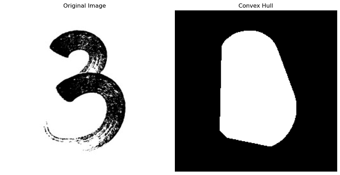
The following example computes the convex hull of a binary image using the convex_hull_image() function.

import numpy as np
from skimage import io, morphology
from matplotlib import pyplot as plt
from skimage.util import invert

# Load an image
image = io.imread("Images/three.jpg", as_gray=True)

# Invert the original image to get the white object.
binary_image = invert(image)

# Compute the convex hull of the binary image
convex_hull = morphology.convex_hull_image(binary_image)

# Create subplots to display the original and the convex hull images side by side
fig, axes = plt.subplots(1, 2, figsize=(10, 5))
ax = axes.ravel()

# Display the original image
ax[0].imshow(image, cmap=plt.cm.gray)
ax[0].set_title('Original Image')
ax[0].set_axis_off()

# Display the black top hat result
ax[1].imshow(convex_hull, cmap=plt.cm.gray)
ax[1].set_title('Convex Hull')
ax[1].set_axis_off()

plt.tight_layout()
plt.show()

Output

On executing the above program, you will get the following output −

Using the skimage.morphology.convex_hull_object() function

The morphology.convex_hull_object() function is used to compute the convex hull image of individual objects in a binary image.

Syntax

Following is the syntax of this function −

skimage.morphology.convex_hull_object(image, *, connectivity=2)

Parameters

• image (M, N) ndarray: This is the input binary image. It should be a 2D array where each element is either 0 or 1.
• connectivity (optional): This parameter determines the neighbors of each pixel. It can take values 1 or 2. In 1-connectivity, only directly adjacent pixels are considered neighbors. In 2-connectivity, diagonally adjacent pixels are also considered neighbors.

Return Value

It returns a binary image of the same shape as the input image.

Example

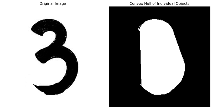
The following example computes the convex hull of individual objects in the binary image using the convex_hull_object() function.

import numpy as np
from skimage import io, morphology
from skimage.util import invert
from matplotlib import pyplot as plt

# Load an image
image = io.imread("Images/three_1.jpg", as_gray=True)

# Invert the original image to get the white object.
binary_image = invert(image)

# Compute the convex hull for individual objects in the binary image
convex_hull_objects = morphology.convex_hull_object(binary_image)

# Create subplots to display the original and the convex hull of individual objects
fig, axes = plt.subplots(1, 2, figsize=(10, 5))
ax = axes.ravel()

ax[0].imshow(image, cmap=plt.cm.gray)
ax[0].set_title('Original Image')
ax[0].set_axis_off()
ax[1].imshow(convex_hull_objects, cmap=plt.cm.gray)
ax[1].set_title('Convex Hull of Individual Objects')
ax[1].set_axis_off()

plt.tight_layout()
plt.show()

Output

On executing the above program, you will get the following output −