Scikit Image - Circular Hough Transform

Quiz

The Circular Hough Transform is an extension of the classic Hough Transform, which is a technique used in image processing and computer vision to detect shapes, particularly lines, circles, and other parametric curves, in an image. The Circular Hough Transform specifically focuses on detecting circles within an image.

In the scikit-image library, you can perform the Circular Hough Transform using the transform.hough_circle() function. This function calculates the Circular Hough Transform and produces an accumulator array in the Hough space, along with the radius values corresponding to the detected circles.

After obtaining the accumulator array, the transform.hough_circle_peaks() function can be used to identify the most significant peaks within the Hough space. These peaks correspond to the detected circles, and the associated radii and coordinates can be utilized to reconstruct the circles in the original image.

Using the transform.hough_circle() function

The transform.hough_circle() function is used to perform a circular Hough transform on an input image.

Syntax

Following is the syntax of this function −

skimage.transform.hough_circle(image, radius, normalize=True, full_output=False)

Parameters

image (ndarray): This is the input image on which the circular Hough transform will be performed. The image is expected to have nonzero values at locations that represent edges. And the shape of the image is (M, N).
radius (scalar or sequence of scalars): This parameter specifies the radii at which the Hough transform will be computed. If you provide floats then those values are converted to integers.
normalize (boolean, optional): This parameter is used to normalize the accumulator using the number of pixels used for drawing the radius.
full_output (boolean, optional): This parameter is used to extend the output size by twice the largest radius to detect centers outside the input image.

Return Value

It returns an accumulator array H, which is a 3D ndarray. The first dimension corresponds to the radius index, the second and third dimensions represent the accumulator array's shape (M + 2R, N + 2R), where M and N are the dimensions of the input image, and R is the radius. If full_output is True, R designates the larger radius.

Example

The following example demonstrates how to use the transform.hough_circle() function to detect a circle in a grayscale image.

import numpy as np
import matplotlib.pyplot as plt
from skimage.transform import probabilistic_hough_line
from skimage.feature import canny
from skimage import io, color

# Load an input image
image = io.imread('Images/Road.jpg', as_gray=True)

# Apply Canny edge detection
edges = canny(image)

# Define the Angles for which to calculate the transform
tested_angles = np.linspace(-np.pi / 2, np.pi / 2, 360, endpoint=False)

# Apply probabilistic Hough line transform
lines = probabilistic_hough_line(edges,  threshold=5, line_length=10, line_gap=3, theta=tested_angles)

# Display the results
fig, axes = plt.subplots(1, 3, figsize=(15, 5), sharex=True, sharey=True)

axes[0].imshow(image, cmap='gray')
axes[0].set_title('Input image')
axes[0].axis('off')

axes[1].imshow(edges, cmap='gray')
axes[1].set_title('Canny edges')
axes[1].axis('off')

axes[2].imshow(edges * 0)
for line in lines:
    p0, p1 = line
    axes[2].plot((p0[0], p1[0]), (p0[1], p1[1]))
axes[2].set_xlim((0, image.shape[1]))
axes[2].set_ylim((image.shape[0], 0))
axes[2].set_title('Probabilistic Hough')
axes[2].axis('off')

plt.tight_layout()
import numpy as np
from skimage.transform import hough_circle
from skimage.draw import circle_perimeter
import matplotlib.pyplot as plt

# Create a blank image
image = np.zeros((200, 200), dtype=np.uint8)

# Draw a circle in the image
rr, cc = circle_perimeter(100, 100, 50)
image[rr, cc] = 255

# Perform circular Hough transform
try_radii = np.arange(5, 60)
accumulator = hough_circle(image, try_radii)

# Find the circle with the maximum accumulator value
ridx, r, c = np.unravel_index(np.argmax(accumulator), accumulator.shape)
detected_center = (r, c)
detected_radius = try_radii[ridx]

print("Output:")
print('Detected Circle Center:',detected_center)
print('Detected Circle Radius:', detected_radius)

# Plot the original image and the detected circle
fig, axes = plt.subplots(1, 2, figsize=(10, 5))
axes[0].imshow(image, cmap='gray')
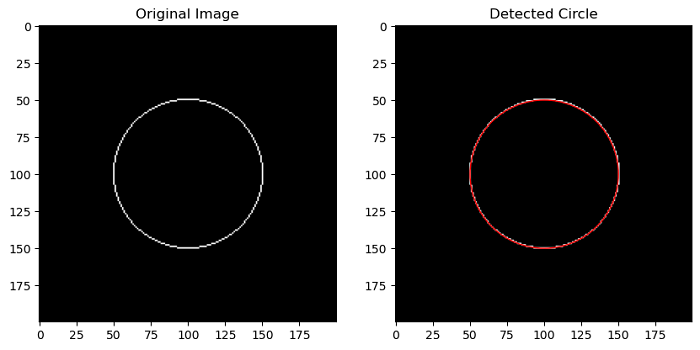
axes[0].set_title('Original Image')

axes[1].imshow(image, cmap='gray')
circle = plt.Circle((detected_center[1], detected_center[0]), detected_radius, color='r', fill=False)
axes[1].add_artist(circle)
axes[1].set_title('Detected Circle')

plt.show()

Output

On executing the above program, you will get the following output −

Output:
Detected Circle Center: (100, 100)
Detected Circle Radius: 50

Using the skimage.transform.hough_circle_peaks() function

The transform.hough_circle_peaks() function is used to identify prominent circles in a circle Hough transform's accumulator space. This function is often used after applying the transform.hough_circle() function to the image to detect circles. It helps to locate and return the most significant circles detected in the Hough space.

Syntax

Following is the syntax of this function −

skimage.transform.hough_circle_peaks(hspaces, radii, min_xdistance=1, min_ydistance=1, threshold=None, num_peaks=inf, total_num_peaks=inf, normalize=False)

Parameters

hspaces (N, M array): This parameter is a collection of Hough spaces returned by the hough_circle() function.
radii (M, array): These are the radii corresponding to the Hough spaces. Each radius corresponds to a particular Hough space.
min_xdistance (optional): It determines the minimum separation distance between centers in the x dimension.
min_ydistance (optional): It determines the minimum separation distance between centers in the y dimension.
threshold (optional): This parameter specifies the minimum intensity of peaks in each Hough space that will be considered as potential circle centers. Default is 0.5 * max(hspace).
num_peaks (int, optional): The maximum number of peaks in each Hough space to consider. If the number of peaks exceeds this value, only the top num_peaks coordinates based on peak intensity will be considered for the corresponding radius.
total_num_peaks (int, optional): The maximum number of peaks across all Hough spaces. If the total number of peaks across all radii exceeds this value, only the top total_num_peaks coordinates based on peak intensity will be returned.
normalize (optional): If set to True, the accumulator is normalized by the radius. This can be useful to sort the prominent peaks.

Return Value

It returns a tuple of four arrays: accum, cx, cy, and rad.

accum: Peak values in the Hough space
cx: X center coordinates of the detected circles.
cy: Y center coordinates of the detected circles.
rad: Radii of the detected circles.

Example

The following example demonstrates how to use the hough_circle_peaks() function with the output of the hough_circle() function.

import numpy as np
from skimage.transform import hough_circle, hough_circle_peaks
from skimage.draw import circle_perimeter
import matplotlib.pyplot as plt

# Create a blank image
image = np.zeros((200, 200), dtype=np.uint8)

# Draw a circle in the image
rr, cc = circle_perimeter(100, 100, 50)
image[rr, cc] = 255

# Perform circular Hough transform
try_radii = np.arange(5, 60)
hspaces = hough_circle(image, try_radii)

# Detect the most prominent circle
accum, cx, cy, rad = hough_circle_peaks(hspaces, try_radii, total_num_peaks=1)

# Print the detected circle parameters
print("Detected Circle:")
print("Center X:", cx[0])
print("Center Y:", cy[0])
print("Radius:", rad[0])

# Visualize the original image and the detected circle
fig, axes = plt.subplots(1, 2, figsize=(10, 5))
axes[0].imshow(image, cmap='gray')
axes[0].set_title('Original Image')

axes[1].imshow(image, cmap='gray')
circle = plt.Circle((cx[0], cy[0]), rad[0], color='r', fill=False)
axes[1].add_artist(circle)
axes[1].set_title('Detected Circle')

plt.show()

Output

On executing the above program, you will get the following output −

Detected Circle:
Center X: 100
Center Y: 100
Radius: 50

Example

The following example demonstrates how to use the probabilistic_hough_line() function to detect lines in an image by specifying the angles(theta) for which to calculate the transform.

import numpy as np
import matplotlib.pyplot as plt
from skimage.transform import probabilistic_hough_line
from skimage.feature import canny
from skimage import io

# Load an input image
image = io.imread('Images/Road.jpg', as_gray=True)

# Apply Canny edge detection
edges = canny(image)

# Define the Angles for which to calculate the transform
tested_angles = np.linspace(-np.pi / 2, np.pi / 2, 360, endpoint=False)

# Apply probabilistic Hough line transform
lines = probabilistic_hough_line(edges,  threshold=5, line_length=10, line_gap=3, theta=tested_angles)

# Display the results
fig, axes = plt.subplots(1, 3, figsize=(15, 5), sharex=True, sharey=True)

axes[0].imshow(image, cmap='gray')
axes[0].set_title('Input image')
axes[0].axis('off')

axes[1].imshow(edges, cmap='gray')
axes[1].set_title('Canny edges')
axes[1].axis('off')

axes[2].imshow(edges * 0)
for line in lines:
    p0, p1 = line
    axes[2].plot((p0[0], p1[0]), (p0[1], p1[1]))
axes[2].set_xlim((0, image.shape[1]))
axes[2].set_ylim((image.shape[0], 0))
axes[2].set_title('Probabilistic Hough')
axes[2].axis('off')

plt.tight_layout()
plt.show()

Output

On executing the above program, you will get the following output −

Print Page