Scikit Image - Total Variation Denoising

Quiz

In image processing, total variation denoising, also referred to as total variation regularization or total variation filtering, is a technique used to reduce noise in an image while preserving its important features. The main objective of this filter is to minimize the total variation norm of the image while maintaining its similarity to the original. Total variation is essentially the L1 norm of the image's gradient.

The scikit-image library provides dedicated functions for applying both the TV Chambolle(denoise_tv_chambolle()) and TV Bregman(denoise_tv_bregman()) denoising algorithms to images.

Using the skimage.restoration.denoise_tv_bregman() function

The restoration.denoise_tv_bregman() function is designed to perform total variation denoising using split-Bregman optimization. This denoising technique aims to find an image u that has reduced total variation compared to the noisy input image f, while still maintaining similarity to f. It is formulated as an optimization problem known as the Rudin--Osher--Fatemi (ROF) minimization problem.

The ROF minimization problem can be expressed as follows −

$$\mathrm{_{u}^{min}\sum_{i=0}^{N-1}\left (\left|\triangledown_{u_{i}} \right| +\frac{\lambda }{2}\left ( f_{i}-u_{i} \right )^{2} \right )}$$

Here, $\lambda$ is a positive parameter, and the cost function consists of two terms: the first term represents total variation, and the second term represents data fidelity. As approaches 0, the total variation term dominates, resulting in a solution with reduced total variation but potentially less similarity to the input data.

Syntax

Following is the syntax of this function −

skimage.restoration.denoise_tv_bregman(image, weight=5.0, max_num_iter=100, eps=0.001, isotropic=True, *, channel_axis=None)

Parameters

The function accepts the following parameters −

image: Input image to be denoised, which should be converted using img_as_float().
weight (optional): Denoising weight, which is equal to $\mathrm{\frac{\lambda }{2}}$. Smaller values of weight result in more denoising, but this may lead to reduced similarity to the original image.
eps (optional): Tolerance value $\mathrm{\varepsilon > 0}$ for the stop criterion. The algorithm stops when $\mathrm{\left\|u_{n}-u_{n-1} \right\|_{2}\lt \varepsilon}$.
max_num_iter (optional): Maximum number of iterations for the optimization process.
isotropic (optional): A boolean parameter that allows you to switch between isotropic and anisotropic total variation (TV) denoising. Isotropic TV denoising is the default behavior.
channel_axis (optional): If None, it assumes that the image is grayscale (single-channel). Otherwise, this parameter specifies which axis of the array corresponds to color channels. This parameter was introduced in version 0.19 of scikit-image.

The function returns the denoised image u as an ndarray.

Example

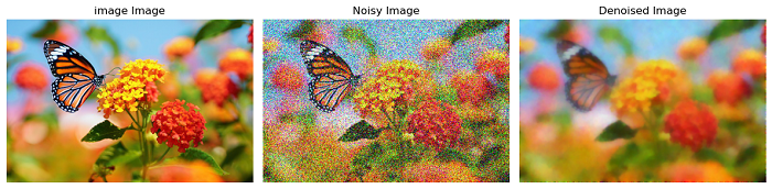
Here's an example of how to use restoration.denoise_tv_bregman() function for performing the total variation denoising using split-Bregman optimization.

import numpy as np
import matplotlib.pyplot as plt
from skimage import io, util
from skimage.restoration import denoise_tv_bregman

# Load a sample image and convert it to floating-point format
image = util.img_as_float(io.imread('Images/butterfly.jpg'))

# Add noise to the image
noisy = image + 0.4 * np.random.standard_normal(image.shape)

# Perform total variation denoising using TV Bregman
denoised_image = denoise_tv_bregman(noisy, weight=0.1, eps=0.0002, max_num_iter=200, channel_axis=-1)

# Visualize the image, noisy, and denoised images
fig, axes = plt.subplots(1, 3, figsize=(12, 4))
ax = axes.ravel()

ax[0].imshow(image, cmap='gray')
ax[0].set_title('image Image')
ax[0].axis('off')

ax[1].imshow(noisy, cmap='gray')
ax[1].set_title('Noisy Image')
ax[1].axis('off')

ax[2].imshow(denoised_image, cmap='gray')
ax[2].set_title('Denoised Image')
ax[2].axis('off')

plt.tight_layout()
plt.show()

Output

Using the skimage.restoration.denoise_tv_chambolle() function

The restoration.denoise_tv_chambolle() function is perform total variation denoising in nD. This denoising technique aims to find an image u that has reduced total variation compared to the noisy input image f, while still maintaining similarity to f. It is formulated as an optimization problem known as the Rudin--Osher--Fatemi (ROF) minimization problem.

The ROF minimization problem can be expressed as follows −

$$\mathrm{_{u}^{min}\sum_{i=0}^{N-1}\left (\left|\triangledown_{u_{i}} \right| +\frac{\lambda }{2}\left ( f_{i}-u_{i} \right )^{2} \right )}$$

Here, $\mathrm{\lambda }$ is a positive parameter, and the cost function consists of two terms: the first term represents total variation, and the second term represents data fidelity. As approaches 0, the total variation term dominates, resulting in a solution with reduced total variation but potentially less similarity to the input data.

Syntax

Following is the syntax of this function −

skimage.restoration.denoise_tv_chambolle(image, weight=0.1, eps=0.0002, max_num_iter=200, *, channel_axis=None)

Parameters

The function accepts the following parameters −

Image (ndarray): Input image to be denoised, which should be converted using img_as_float().
weight (optional): Denoising weight, which is equal to $\mathrm{\frac{1}{\lambda }}$. Therefore, the greater the weight, the more aggressive the denoising, but it may come at the expense of fidelity to the original image.
eps (float, optional): Tolerance value ϵ > 0 for the stop criterion. The algorithm stops when |E_{n-1} - E_n| < \varepsilon * E_0`.
max_num_iter (optional): Maximum number of iterations for the optimization process.
channel_axis (optional): If None, it assumes that the image is grayscale (single-channel). Otherwise, this parameter specifies which axis of the array corresponds to color channels. This parameter was introduced in version 0.19 of scikit-image.

The function returns the denoised image u as an ndarray.

It's important to ensure that the channel_axis parameter is set appropriately, especially when working with color images.

The principle of total variation denoising, which this function implements, is to minimize the total variation of an image. Total variation can be thought of as the integral of the norm of the image gradient. In practice, total variation denoising tends to produce images with a cartoon-like appearance, that is, piecewise-constant images.

Example

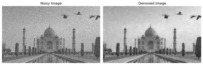
Here is an examples of using the restoration.denoise_tv_chambolle() function on a 2D image.

import numpy as np
import matplotlib.pyplot as plt
from skimage import color, io, util
from skimage.restoration import denoise_tv_chambolle

# Load theinput image and convert it to grayscale
image = color.rgb2gray(io.imread('Images/Tajmahal.jpg'))
image = util.img_as_float(image)

# Add noise to the image
rng = np.random.default_rng()
image += 0.5 * image.std() * rng.standard_normal(image.shape)

# Denoise the noisy image using TV Chambolle denoising with a specified weight.
denoised_image = denoise_tv_chambolle(image, weight=0.1)

# Visualize the noisy, and denoised images
fig, axes = plt.subplots(1, 2, figsize=(10, 5))
ax = axes.ravel()

ax[0].imshow(image, cmap='gray')
ax[0].set_title('Noisy Image')
ax[0].axis('off')

ax[1].imshow(denoised_image, cmap='gray')
ax[1].set_title('Denoised Image')
ax[1].axis('off')

plt.tight_layout()
plt.show()

Output

Example

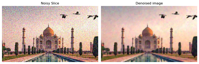
Let's apply the restoration.denoise_tv_chambolle() function on a 3D image.

import numpy as np
import matplotlib.pyplot as plt
from skimage import io, util
from skimage.restoration import denoise_tv_chambolle

# Load the input image
image = util.img_as_float(io.imread('Images/Tajmahal.jpg'))

# Add noise to the image
rng = np.random.default_rng()
image += 0.5 * image.std() * rng.standard_normal(image.shape)

# Denoise the noisy image using TV Chambolle denoising with a specified weight.
denoised_image = denoise_tv_chambolle(image, weight=0.1, channel_axis=-1)

# Visualize the noisy, and denoised image
fig, axes = plt.subplots(1, 2, figsize=(10, 5))
ax = axes.ravel()

ax[0].imshow(image, cmap='gray')
ax[0].set_title('Noisy Slice')
ax[0].axis('off')

ax[1].imshow(denoised_image, cmap='gray')
ax[1].set_title('Denoised image')
ax[1].axis('off')

plt.tight_layout()
plt.show()

Output

Print Page