Scikit Image - Dense DAISY Feature Description

Quiz

The Dense DAISY feature description is a local image descriptor that relies on gradient orientation histograms, similar to the SIFT descriptor. However, it is designed in such a way that it enables rapid and dense extraction of features. This characteristic makes it particularly valuable for tasks such as generating bag-of-features image representations.

The scikit image library provides a dedicated function within its feature module for extracting Dense DAISY feature descriptors from grayscale images.

Using the skimage.feature.daisy() function

The skimage.feature.daisy() function is used to extract DAISY feature descriptors from a grayscale image. DAISY is a feature descriptor similar to SIFT (Scale-Invariant Feature Transform) but is designed for fast dense extraction, making it suitable for bag-of-features image representations.

Syntax

Following is the syntax of this function −

skimage.feature.daisy(image, step=4, radius=15, rings=3, histograms=8, orientations=8, normalization='l1', sigmas=None, ring_radii=None, visualize=False)

Parameters

Here are the details of the parameters −

image: Input grayscale image (M, N) for which DAISY feature descriptors are extracted.
step (int, optional): It determines the distance between descriptor sampling points.
radius (int, optional): it specifies the radius (in pixels) of the outermost ring.
rings (int, optional): Number of rings. It determines how many concentric rings are created around each sampling point.
histograms (int, optional): Number of histograms sampled per ring.
orientations (int, optional): Number of orientations (bins) per histogram.
normalization (optional): Specifies how to normalize the descriptors. It can be one of the following options −
- 'l1': L1-normalization of each descriptor.
- 'l2': L2-normalization of each descriptor.
- 'daisy': L2-normalization of individual histograms.
- 'off': Disable normalization.
sigmas (1D array of float, optional): Standard deviation of spatial Gaussian smoothing for the center histogram and each ring of histograms. This parameter controls the amount of spatial smoothing applied to the histograms. Specifying sigmas overrides the following parameter: rings = len(sigmas) - 1
ring_radii (1D array of int, optional): Radius (in pixels) for each ring. Specifying ring_radii overrides the following two parameters.

rings = len(ring_radii) radius = ring_radii[-1]

If both sigmas and ring_radii parameters are given, they must satisfy the following predicate since no radius is needed for the center histogram.

len(ring_radii) == len(sigmas) + 1

visualize (bool, optional): If set to True, it generates a visualization of the DAISY descriptors.

The function returns a grid of DAISY descriptors for the given image as a NumPy array with dimensions (P, Q, R), where −

P = ceil((M - radius * 2) / step)
Q = ceil((N - radius * 2) / step)
R = (rings * histograms + 1) * orientations

Additionally, if visualize is set to True, it also returns a visualization of the DAISY descriptors as a NumPy array with dimensions (M, N, 3).

Example

Here is an example that applies the DAISY descriptors with default parameters, and displays the shape of the descriptors array along with count of the total number of DAISY descriptors extracted.

import numpy as np
from skimage import io, feature

# Load an example grayscale image
image = io.imread('Images/image5.jpg', as_gray=True)

# apply the DAISY descriptors with default parameters
descriptors = feature.daisy(image)

# Display the results 
print("Shape of descriptors:", descriptors.shape)
print("Total DAISY descriptors extracted:", descriptors.shape[0] * descriptors.shape[1])

Output

Shape of descriptors: (82, 94, 200)
Total DAISY descriptors extracted: 7708

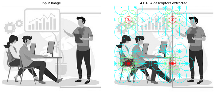
Example

The following example demonstrates how to extract DAISY features from a grayscale image.

from skimage.feature import daisy
from skimage import io
import matplotlib.pyplot as plt

# Load a sample grayscale image
image = io.imread('Images/image5.jpg', as_gray=True)

# Extract DAISY features with visualization
descs, descs_img = daisy(image, step=180, radius=58, rings=2, histograms=6,
   orientations=8, visualize=True)

# Create subplots for input and output visualization
fig, (ax1, ax2) = plt.subplots(1, 2, figsize=(12, 5))

# Display the original input image
ax1.imshow(image, cmap='gray')
ax1.set_title("Input Image")
ax1.axis("off")

# Display the DAISY descriptors visualization
ax2.imshow(descs_img)
ax2.set_title(f"{descs.shape[0] * descs.shape[1]} DAISY descriptors extracted")
ax2.axis("off")

plt.tight_layout()
plt.show()

Output

Print Page