Scikit Image - Canny Edge Detection

Quiz

The Canny edge detection is a multi-stage algorithm designed for identifying edges in images. Initially, it employs a Gaussian-based filter to compute gradient intensity, effectively reducing the impact of image noise. Then, it refines potential edges by thinning them down to 1-pixel-wide curves, selectively removing non-maximum gradient magnitude pixels. Finally, edge pixels are determined through the application of hysteresis thresholding on the gradient magnitude.

The Canny algorithm offers three adjustable parameters: the Gaussian filter's width (which should be increased for noisier images), as well as the low and high thresholds utilized during hysteresis thresholding.

The algorithm follows the below steps to detect edges in an image −

Smoothing the Image: The first step involves applying a Gaussian filter to the input image with sigma width.
Gradient Calculation: The horizontal and vertical gradients of the smoothed image are calculated using Sobel operators. The edge strength is the norm of the gradient.
Edge Thinning: In this step, potential edges are thinned to 1-pixel wide curves. To do this, the algorithm calculates the normal direction at each pixel by analyzing the signs and relative magnitudes of the gradients obtained using the X-Sobel and Y-Sobel operators. This categorizes the points into four groups: horizontal, vertical, diagonal, and antidiagonal. Then, the algorithm looks in both the normal and reverse directions to see if the gradient magnitudes are greater than the point in question. Interpolation may be used to obtain a mix of points along the edge, rather than simply selecting the closest one.
Hysteresis Thresholding: Initially, all points above the high threshold are labeled as edges. Then, the algorithm recursively labels any point above the low threshold that is 8-connected (connected in eight directions: horizontally, vertically, and diagonally) to a labeled edge point as an edge. This process helps connect weaker edge segments to stronger ones, creating a continuous edge map.

The scikit-image library provides the canny() function within its feature module to perform Canny edge detection on images.

Using the skimage.feature.canny() function

The canny() function in the skimage feature module is used to filter edges in a grayscale input image using the Canny algorithm.

Syntax

Following is the syntax of this function −

skimage.feature.canny(image, sigma=1.0, low_threshold=None, high_threshold=None, mask=None, use_quantiles=False, *, mode='constant', cval=0.0)

Parameters

Here's an explanation of its parameters −

image (2D array): This is the grayscale input image in which to detect edges.
sigma (float, optional): This parameter specifies the standard deviation of the Gaussian filter.
low_threshold (float, optional): This sets the lower bound for hysteresis thresholding, which is a part of the Canny edge detection process. If not provided (None), it is set to 10% of the maximum value of the data type of the input image.
high_threshold (float, optional): This sets the upper bound for hysteresis thresholding. If not provided (None), it is set to 20% of the maximum value of the data type of the input image.
mask (array, dtype=bool, optional): A mask as a boolean array to limit the application of the Canny edge detection algorithm to a specific area of the image.
use_quantiles (bool, optional): If set to True, this parameter treats low_threshold and high_threshold as quantiles of the edge magnitude image rather than absolute values. If True, the thresholds should be in the range [0, 1].
mode (str, optional): This parameter determines how the array borders are handled during Gaussian filtering. It specifies the type of padding to be used at the image borders. The options are: 'reflect', 'constant', 'nearest', 'mirror', and 'wrap'.
cval (float, optional): If the mode is set to 'constant', this parameter specifies the value to fill past the edges of the input image during Gaussian filtering.

The function returns a 2D array representing the binary edge map, which is an image where the edges are represented as binary values (usually 0 for no edge and 1 for an edge).

Example

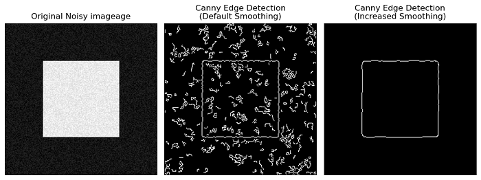
Here is an example that demonstrates how to use the Canny edge detection (canny()) function from the skimage.feature module to detect edges in an image.

import numpy as np
from skimage import feature
import matplotlib.pyplot as plt

# Generate noisy imageage of a square
rng = np.random.default_rng()
image = np.zeros((256, 256))
image[64:-64, 64:-64] = 1
image += 0.2 * rng.random(image.shape)

# First trial with the Canny filter, with the default smoothing
edges1 = feature.canny(image)

# Increase the smoothing for better results
edges2 = feature.canny(image, sigma=3)

# Visualize the original, noisy, and results (Canny Edge Detection)
fig, axes = plt.subplots(1, 3, figsize=(10, 5))

# Original Noisy imageage
axes[0].imshow(image, cmap='gray')
axes[0].set_title('Original Noisy imageage')
axes[0].axis('off')

# Canny Edge Detection (Default Smoothing)
axes[1].imshow(edges1, cmap='gray')
axes[1].set_title('Canny Edge Detection&bsol;n(Default Smoothing)')
axes[1].axis('off')

# Canny Edge Detection (Increased Smoothing)
axes[2].imshow(edges2, cmap='gray')
axes[2].set_title('Canny Edge Detection&bsol;n(Increased Smoothing)')
axes[2].axis('off')

plt.tight_layout()
plt.show()

Output

Example

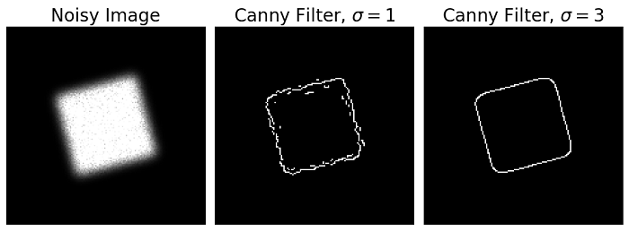
Let's take another noisy image to apply the Canny edge detection algorithm to it with two different values of sigma, and display the original noisy image along with the Canny edge detection results.

import numpy as np
import matplotlib.pyplot as plt
from scipy import ndimage as ndi
from skimage.util import random_noise
from skimage import feature

# Generate a noisy image of a square
image = np.zeros((128, 128), dtype=float)
image[32:-32, 32:-32] = 1

# Rotate the square by 15 degrees
image = ndi.rotate(image, 15, mode='constant')

# Apply Gaussian smoothing to the image
image = ndi.gaussian_filter(image, 4)

# Add speckle noise to the image
image = random_noise(image, mode='speckle', mean=0.1)

# Compute the Canny filter for two values of sigma
edges1 = feature.canny(image)
edges2 = feature.canny(image, sigma=3)

# Display the results
fig, ax = plt.subplots(nrows=1, ncols=3, figsize=(10, 5))

# Plot the noisy image
ax[0].imshow(image, cmap='gray')
ax[0].set_title('Noisy Image', fontsize=20)

# Plot the result of Canny filter with sigma=1
ax[1].imshow(edges1, cmap='gray')
ax[1].set_title(r'Canny Filter, $&bsol;sigma=1$', fontsize=20)

# Plot the result of Canny filter with sigma=3
ax[2].imshow(edges2, cmap='gray')
ax[2].set_title(r'Canny Filter, $&bsol;sigma=3$', fontsize=20)

for a in ax:
   a.axis('off')

fig.tight_layout()
plt.show()

Output

Print Page