Scikit Image - Exposure

Quiz

Exposure in an image indicates whether the image appears excessively dark, too bright, or well-balanced in terms of brightness. This characteristic can be estimated by analysing the histogram of intensity values across all the pixels of the image. Enhancing image exposure is a fundamental task in image processing.

Exposure adjustment techniques such as gamma correction, logarithmic correction, and sigmoid correction are used to enhance the quality and visual appeal of images.

The scikit-image library in Python provides the adjust_gamma(), adjust_log(), and adjust_sigmoid() functions in the exposure module. These functions useful to easily apply exposure adjustment techniques like gamma correction, logarithmic correction, and sigmoid correction to images.

Using the skimage.exposure.adjust_gamma() function

The exposure.adjust_gamma() function is used to perform Gamma Correction (also known as Power Law Transform) on an input image. This transformation is applied pixel by pixel, following the formula O = I**gamma, after each pixel is scaled to the range from 0 to 1.

Syntax

Following is the syntax of this function −

skimage.exposure.adjust_gamma(image, gamma=1, gain=1)

Parameters

image: The input image in the form of an ndarray.
gamma: A non-negative real number (default value: 1). This parameter determines the exponent for the power-law transformation.
gain: An optional constant multiplier (default value: 1).

Return Value

It returns the gamma-corrected output image as an ndarray.

It is important to note that, if gamma is greater than 1, the histogram will shift towards the left, resulting in a darker output image compared to the input image. And if gamma is less than 1, the histogram will shift towards the right, leading to a brighter output image compared to the input image.

Example

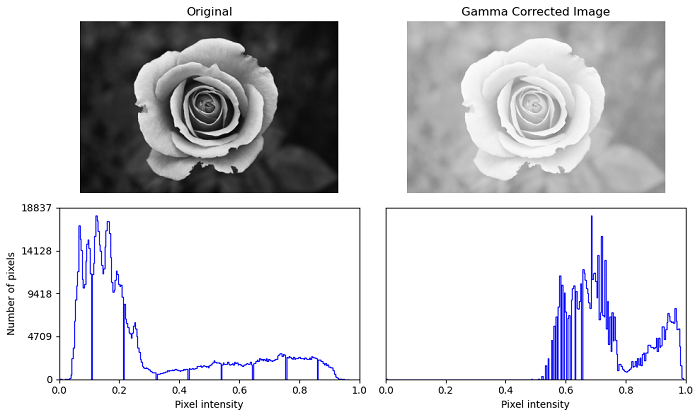
The following example demonstrates how gamma correction affects the appearance and pixel intensity distribution of an image. The original and gamma-corrected images, along with their histograms, are displayed side by side for visual comparison.

from skimage import io, exposure, img_as_float
import matplotlib.pyplot as plt
import numpy as np

# Load an example image
image = io.imread('Images/black rose.jpg')
image = img_as_float(image)

# Apply gamma correction with gamma = 0.2
gamma_corrected = exposure.adjust_gamma(image, 0.2)

# Display the original and gamma_corrected images side by side
fig, axes = plt.subplots(2, 2, figsize=(10, 6))
ax = axes.ravel()

ax[0].imshow(image, cmap=plt.cm.gray)
ax[0].set_title('Original')
ax[0].set_axis_off()

ax[1].imshow(gamma_corrected, cmap=plt.cm.gray)
ax[1].set_title('Gamma Corrected Image')
ax[1].set_axis_off()

ax[2].hist(image.ravel(), bins=256, histtype='step', color='blue')
ax[2].set_xlim(0, 1)
ax[2].set_xlabel('Pixel intensity')
ax[2].set_yticks([])
ax[2].set_ylabel('Number of pixels')
y_min, y_max = ax[2].get_ylim()
ax[2].set_yticks(np.linspace(0, y_max, 5))

ax[3].hist(gamma_corrected.ravel(), bins=256, histtype='step', color='blue')
ax[3].set_xlim(0, 1)
ax[3].set_xlabel('Pixel intensity')
ax[3].set_yticks([])

plt.tight_layout()
plt.show()

Output

On executing the above program, you will get the following output −

Using the skimage.exposure.adjust_log() function

The function exposure.adjust_log(image, gain=1, inv=False) applies logarithmic correction to an input image. This correction transforms each pixel in the input image according to the following equations:

For logarithmic correction:

O = gain * log(1 + I)

For inverse logarithmic correction:

O = gain * (2**I - 1)

In both cases, the transformation is applied after scaling each pixel to the range between 0 and 1.

Syntax

Following is the syntax of this function −

skimage.exposure.adjust_log(image, gain=1, inv=False)

Parameters

image: The input image as an ndarray.
gain: An optional constant multiplier (default value: 1).
inv: If True, inverse logarithmic correction is performed; otherwise, the correction will be logarithmic (default value: False).

Return Value

It returns the logarithmic corrected image as an ndarray.

Example

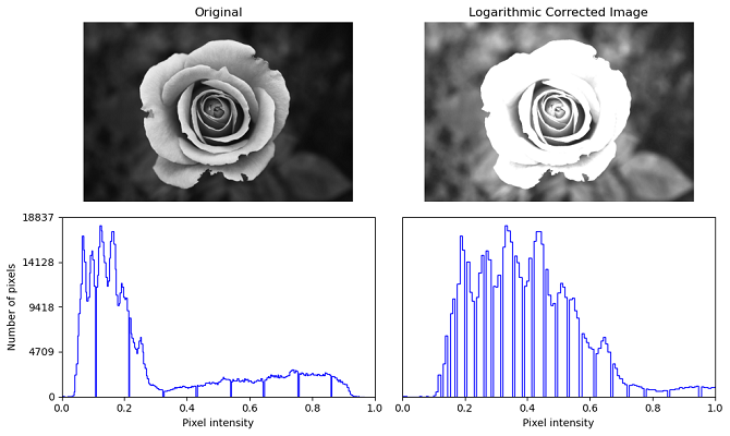
The following example demonstrates how logarithmic correction affects the appearance and pixel intensity distribution of an image. The original and logarithmic corrected images, along with their histograms, are displayed side by side for visual comparison.

from skimage import io, exposure, img_as_float
import matplotlib.pyplot as plt
import numpy as np

# Load an example image
image = io.imread('Images/black_rose.jpg')
image = img_as_float(image)

# Apply Logarithmic correction with gain = 2
log_corrected = exposure.adjust_log(image, gain=2)

# Display the original and Logarithmic corrected images side by side
fig, axes = plt.subplots(2, 2, figsize=(10, 6))
ax = axes.ravel()

ax[0].imshow(image, cmap=plt.cm.gray)
ax[0].set_title('Original')
ax[0].set_axis_off()

ax[1].imshow(log_corrected, cmap=plt.cm.gray)
ax[1].set_title('Logarithmic Corrected Image')
ax[1].set_axis_off()

ax[2].hist(image.ravel(), bins=256, histtype='step', color='blue')
ax[2].set_xlim(0, 1)
ax[2].set_xlabel('Pixel intensity')
ax[2].set_yticks([])
ax[2].set_ylabel('Number of pixels')
y_min, y_max = ax[2].get_ylim()
ax[2].set_yticks(np.linspace(0, y_max, 5))

ax[3].hist(log_corrected.ravel(), bins=256, histtype='step', color='blue')
ax[3].set_xlim(0, 1)
ax[3].set_xlabel('Pixel intensity')
ax[3].set_yticks([])

plt.tight_layout()
plt.show()

Output

On executing the above program, you will get the following output −

Using the skimage.exposure.adjust_sigmoid() function

The function skimage.exposure.adjust_sigmoid(image, cutoff=0.5, gain=10, inv=False) performs Sigmoid Correction on an input image. Sigmoid correction is also known as Contrast Adjustment. This correction transforms each pixel in the input image using the following equation:

O = 1 / (1 + exp*(gain * (cutoff - I)))

This transformation is applied after scaling each pixel to the range between 0 and 1.

Syntax

Following is the syntax of this method −

skimage.exposure.adjust_sigmoid(image, cutoff=0.5, gain=10, inv=False)

Parameters

image: The input image in the form of an ndarray.
cutoff: An optional parameter that determines the cutoff point of the sigmoid function, shifting the characteristic curve horizontally (default value: 0.5).
gain: An optional constant multiplier that affects the exponential power of the sigmoid function (default value: 10).
inv: An optional boolean parameter. If True, it returns the negative sigmoid correction; otherwise, it performs the regular sigmoid correction (default value: False).

Return Value

It returns the sigmoid corrected image as an ndarray.

Example

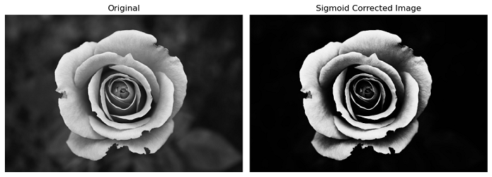
Here's an example of how to use the exposure.adjust_sigmoid() function to perform sigmoid correction on an image.

from skimage import io, exposure
import matplotlib.pyplot as plt

# Load an example image
image = io.imread('Images/black_rose.jpg')

# Apply sigmoid correction
sigmoid_corrected = exposure.adjust_sigmoid(image, cutoff=0.6, gain=10)

# Display the original and sigmoid-corrected images
fig, axes = plt.subplots(1, 2, figsize=(10, 5))
ax = axes.ravel()

ax[0].imshow(image, cmap=plt.cm.gray)
ax[0].set_title('Original')
ax[0].set_axis_off()

ax[1].imshow(sigmoid_corrected, cmap=plt.cm.gray)
ax[1].set_title('Sigmoid Corrected Image')
ax[1].set_axis_off()

plt.tight_layout()
plt.show()

Output

On executing the above program, you will get the following output −

Print Page