Scikit Image - Marching Cubes

Quiz

Marching cubes is a 3D algorithm used to create a surface mesh from a 3D volume. This can be conceptualized as a 3D generalization of isolines on topographical or weather maps. It works by iterating through the volume, identifying regions that meet a certain level of interest, and then creating triangles to build a 3D mesh. This algorithm requires two main inputs: the 3D data volume and an isosurface value. For instance, in CT imaging Hounsfield units of +700 to +3000 represent bone density within the CT data. So, one potential input would be a reconstructed CT set of data and the value +700, to extract a mesh for regions of bone or bone-like density. The result is a mesh consisting of vertices and triangular faces.

The scikit image library provides the marching_cubes() function within its measure module to work with 3D volumetric data.

Using the skimage.measure.marching_cubes() function

The marching_cubes() function is an implementation of the Marching Cubes algorithm designed to identify surfaces within 3D volumetric data. Unlike the approach by Lorensen et al., this implementation follows the algorithm by Lewiner et al. This choice brings several advantages: it's faster, resolves ambiguities, and ensures topologically correct results. Therefore, when working with 3D data, using marching_cubes() with the Lewiner et al. method is generally the better choice.

Syntax

Following is the syntax of this function −

skimage.measure.marching_cubes(volume, level=None, *, spacing=(1.0, 1.0, 1.0), gradient_direction='descent', step_size=1, allow_degenerate=True, method='lewiner', mask=None)

Parameters

The function accepts the following parameters −

volume (M, N, P) array: Input 3D data volume from which isosurfaces will be extracted. It Will internally be converted to float32 if necessary.
level (float, optional): Contour value to search for isosurfaces in the volume. Default is the average of the minimum and maximum values in the volume.
spacing (length-3 tuple of floats, optional): Voxel spacing in spatial dimensions corresponding to numpy array indexing dimensions (M, N, P) as in the volume.
gradient_direction (string, optional): Specifies whether the mesh is generated from an isosurface with gradient descent or ascent.
step_size (int, optional): Step size in voxels. The default value is 1. Larger steps yield faster but coarser results. The result will always be topologically correct.
allow_degenerate (bool, optional): Determines whether degenerate (i.e. zero-area) triangles are allowed in the output mesh. The default is True. If False, degenerate triangles are removed, making the algorithm slower.
method ({'lewiner', 'lorensen'}, optional): Specifies the algorithm to use, either Lewiner et al. or the Lorensen et al. method.
mask (M, N, P) array, optional: Boolean array to restrict the computation to certain regions of the volume. The marching cube algorithm will be computed only on True elements, saving computational time and allowing for finite surfaces.

Function returns −

verts (V, 3) array: Spatial coordinates for V unique mesh vertices. Coordinate order matches the input volume (M, N, P).
faces (F, 3) array: Defines triangular faces via referencing vertex indices from verts. Each face has exactly three indices.
normals (V, 3) array: The normal direction at each vertex, as calculated from the data.
values (V, ) array: Gives a measure for the maximum value of the data in the local region near each vertex, useful for applying a colormap to the mesh in visualization tools.

Example

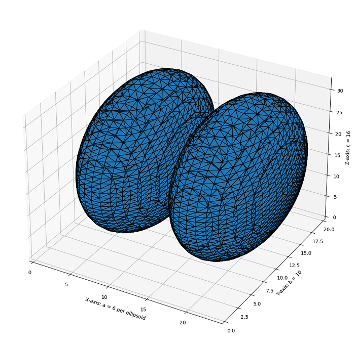
The following example demonstrates how to use the Marching Cubes algorithm to generate and visualize a 3D mesh from a 3D dataset.

import numpy as np
import matplotlib.pyplot as plt
from mpl_toolkits.mplot3d.art3d import Poly3DCollection
from skimage import measure
from skimage.draw import ellipsoid

# Generate a level set of two identical ellipsoids in 3D
ellipsoid_base = ellipsoid(6, 10, 16, levelset=True)

# Create a larger dataset by stacking two identical ellipsoids along the z-axis
ellipsoid_double = np.concatenate((ellipsoid_base[:-1, ...], ellipsoid_base[2:, ...]), axis=0)

# Extract the surface mesh of the ellipsoids using marching cubes
vertices, faces, normals, values = measure.marching_cubes(ellipsoid_double, 0)

# Create a 3D plot for visualization
fig = plt.figure(figsize=(10, 10))
ax = fig.add_subplot(111, projection='3d')

# Create a collection of triangles from vertices and faces
mesh = Poly3DCollection(vertices[faces])
mesh.set_edgecolor('k')
ax.add_collection3d(mesh)

# Set labels and axis limits
ax.set_xlabel("X-axis: a = 6 per ellipsoid")
ax.set_ylabel("Y-axis: b = 10")
ax.set_zlabel("Z-axis: c = 16")
ax.set_xlim(0, 24)  
ax.set_ylim(0, 20)  
ax.set_zlim(0, 32)  

plt.tight_layout()
plt.show()

Output

Example

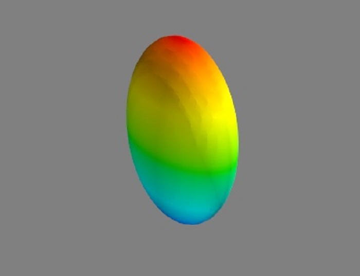
Here is an example that demonstrates how to visualize the output of the Marching Cubes algorithm using the Mayavi package.

from mayavi import mlab
from skimage.measure import marching_cubes
import matplotlib.pyplot as plt
from skimage import measure
from skimage.draw import ellipsoid

# Generate an identical ellipsoids in 3D
ellipsoid_base = ellipsoid(6, 10, 16, levelset=True)

# Extract the surface mesh of the ellipsoids using marching cubes
verts, faces, _, _ = measure.marching_cubes(ellipsoid_base, 0.0)

# Extract coordinates from vertices
x_coords = [vert[0] for vert in verts]
y_coords = [vert[1] for vert in verts]
z_coords = [vert[2] for vert in verts]

# Create a 3D triangular mesh using Mayavi
mlab.triangular_mesh(x_coords, y_coords, z_coords, faces)

# Display the 3D mesh
mlab.show()

Output

Print Page