Scikit Image - Conversion from CIE-LAB Colorspace

Quiz

The CIELAB color space also referred to as L*a*b*, is a color space defined by the International Commission on Illumination (abbreviated CIE) in 1976. The LAB stands for Lightness, position between red and green, and position between yellow and blue.

It represents colors using three values: L* for perceptual lightness, and a* and b* for the four unique colors of human vision: red, green, blue, and yellow. The primary goal of CIELAB was to create a perceptually uniform color space, where a specific numerical change corresponds to a similar perceived change in color. It is widely used in various applications, including color image processing, computer vision, color management, and detecting small differences in color.

The Scikit-Image library provides functions like color.lab2rgb(), color.lab2lch(), and color.lab2xyz() to do conversions from LAB color space to RGB, LCH, and XYZ color spaces.

Converting CIE-LAB image to RGB

The skimage.color.lab2rgb() function is used to perform the conversion of an image from the CIE-LAB color space to the sRGB color space.

Syntax

Following is the syntax of this function −

skimage.color.lab2rgb(lab, illuminant='D65', observer='2', *, channel_axis=-1)

The method accepts the following parameters −

lab (array_like): The input image in CIE-LAB color space. The shape of the array should be at least 2-D with the last dimension having a size of 3, representing the CIE-LAB channels.
Illuminant (str, optional): Representing the name of the illuminant {A, B, C, D50, D55, D65, D75, E}. The default value is 'D65'.
observer (str, optional): Representing the aperture angle of the observer {2, 10, R}. The default value is '2'.
channel_axis: This parameter indicates which axis of the array corresponds to the channels. By default, it is set to -1, corresponding to the last axis.

The method returns a ndarray representing the output image in sRGB color space. The dimensions of the output array are the same as the input array.

And the method will raise the ValueError, if the lab input is not at least 2-D with a shape of (..., 3, ...), indicating the presence of the three channels.

Example

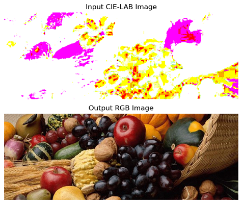
The following example demonstrates the conversion of an image in CIE-LAB color space to XYZ color space using color.lab2rgb() method.

import numpy as np
from skimage import color, io
import matplotlib.pyplot as plt

# Read an RGB image as lab
lab_image = color.rgb2lab(io.imread('Images/Fruits.jpg'))

# Convert LAB to RGB
rgb_image = color.lab2rgb(lab_image)

# Display the LAB and RGB images using Matplotlib
fig, axes = plt.subplots(nrows=2, ncols=1, figsize=(10, 5))

axes[0].imshow(lab_image)
axes[0].set_title('Input CIE-LAB Image')
axes[0].axis('off')

axes[1].imshow(rgb_image)
axes[1].set_title('Output RGB Image')
axes[1].axis('off')

plt.tight_layout()
plt.show()

Output

On executing the above program, you will get the following output −

Converting CIE-LAB image to LCH

The skimage.color.lab2lch() method is used to perform the conversion of an image from the CIE-LAB color space to the CIE-LCh color space. The CIE-LCh color space is the cylindrical representation of the CIE-LAB (Cartesian) color space.

Syntax

Following is the syntax of this function −

skimage.color.lab2lch(lab, *, channel_axis=-1)

The method accepts the following parameters −

lab (array_like): The input image in CIE-LAB color space. The shape of the array should be at least 3-D with the last dimension having a size of 3, representing the CIE-LAB channels.
channel_axis: This parameter indicates which axis of the array corresponds to the channels. By default, it is set to -1, which corresponds to the last axis.

The method returns a ndarray representing the output image in CIE-LCh format. The dimensions of the output array are the same as the input array. And the method will raise the ValueError if the lab input does not have at least 3 channels.

It's important to note that the lab2lch function assumes the Hue channel (i.e., h) is expressed as an angle in the range (0, 2*pi).

Example

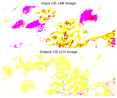
The following example demonstrates the conversion of an image from CIE-LAB color space to CIE-LCH color space using color.lab2lch() method.

import numpy as np
from skimage import color, io, util
import matplotlib.pyplot as plt

# Read a RGB image 
rgb_image = io.imread('Images/Fruits.jpg')
# get the LAB image from an RGB image
lab_image = color.rgb2lab(rgb_image)

# Convert LAB to LCH
lch_image = color.lab2lch(lab_image)

# Display the LAB and LCH images using Matplotlib
fig, axes = plt.subplots(nrows=2, ncols=1, figsize=(10, 5))

axes[0].imshow(lab_image)
axes[0].set_title('Input CIE-LAB Image')
axes[0].axis('off')

axes[1].imshow(lch_image)
axes[1].set_title('Output CIE-LCH Image')
axes[1].axis('off')

plt.tight_layout()
plt.show()

Output

Converting CIE-LAB image to xyz color space

The skimage.color.lab2xyz() function is used to perform the conversion of an image from the CIE-LAB color space to the XYZ color space.

Syntax

Following is the syntax of this function −

skimage.color.lab2xyz(lab, illuminant='D65', observer='2', *, channel_axis=-1)

The method accepts the following parameters −

lab (array_like): The input image in CIE-LAB color space. The shape of the array should be at least 2-D with the last dimension having a size of 3, representing the CIE-LAB channels.
Illuminant (str, optional): Representing the name of the illuminant {A, B, C, D50, D55, D65, D75, E}. The default value is 'D65'.
observer (str, optional): Representing the aperture angle of the observer {2, 10, R}. The default value is '2'.
channel_axis: This parameter indicates which axis of the array corresponds to the channels. By default, it is set to -1, which corresponds to the last axis.

The method returns a ndarray representing the output image in XYZ color space. The dimensions of the output array are the same as the input array.

And the method will raise the following exceptions −

ValueError: If the lab input is not at least 2-D with a shape of (..., 3, ...), indicating the presence of the three channels.
ValueError: If either the illuminant or the observer angle is unsupported or unknown.
UserWarning: If any of the pixels have invalid values (Z < 0) in the XYZ color space.

Example

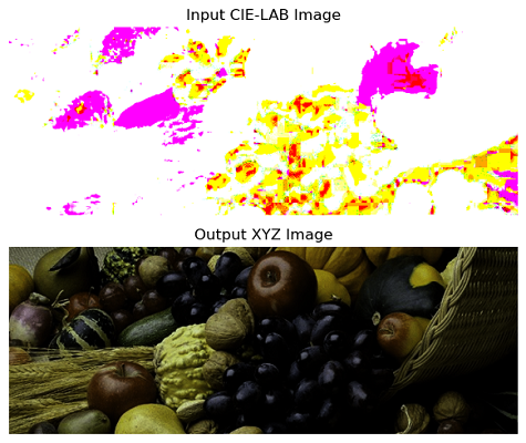
The following example demonstrates the conversion of an image from CIE-LAB color space image to an image in XYZ color space using color.lab2xyz() method.

import numpy as np
from skimage import color, io
import matplotlib.pyplot as plt

# Read a RGB image as lab
lab_image = color.rgb2lab(io.imread('Images/Fruits.jpg'))

# Convert LAB to XYZ
xyz_image = color.lab2xyz(lab_image)

# Display the LAB and XYZ images using Matplotlib
fig, axes = plt.subplots(nrows=2, ncols=1, figsize=(10, 5))

axes[0].imshow(lab_image)
axes[0].set_title('Input CIE-LAB Image')
axes[0].axis('off')

axes[1].imshow(xyz_image)
axes[1].set_title('Output XYZ Image')
axes[1].axis('off')

plt.tight_layout()
plt.show()

Output

On executing the above program, you will get the following output −

Print Page