Scikit Image - Black and White Tophat Morphologies

---

---

Black and white top-hat morphologies are image-processing operations used to enhance or extract features from an image. They are based on morphological operations and are often used in tasks like image enhancement, background subtraction, and feature extraction.

The white top hat of an image is defined as the difference between the original image and its morphological opening (white top hat = image - opening). In other words, it reveals the bright regions of the image that are smaller than the provided footprint.

Whereas the black top hat operation is defined as the difference between the morphological closing of an image and the original image (black hat = closing - image). It highlights the dark spots in the image that are smaller than the specified footprint. Dark spots in the original image are converted to bright spots after performing the black tophat operation.

The scikit image library provides the morphology.white_tophat() and morphology.black_tophat() functions to perform these morphological operations on images.

Using the skimage.morphology.white_tophat() function

The morphology.white_tophat()function performs the white tophat operation on an image.

Syntax

Following is the syntax of this function −

skimage.morphology.white_tophat(image, footprint=None, out=None)

Parameters

• image (ndarray): The input image on which the white top hat operation will be performed.
• footprint (ndarray or tuple, optional): The neighborhood expressed as a 2-D array of 1s and 0s. If None is provided, a cross-shaped footprint (connectivity=1) is used. You can also specify a custom footprint as a sequence of smaller footprints, which can help reduce the computational cost for certain footprints.
• out (ndarray, optional): The output array where the result of the white top hat operation will be stored. If None is passed, a new array will be allocated for the result.

Return Value

It returns a ndarray representing the morphological white tophat of the input image, and the output array has the same shape and data type as the input image.

Example

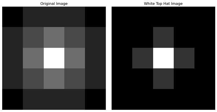
Here's an example of how to use the white_tophat() function.

import numpy as np
import matplotlib.pyplot as plt
from skimage.morphology import white_tophat, square

# Create an example input image
bright_on_gray = np.array([[2, 3, 3, 3, 2],
                           [3, 4, 5, 4, 3],
                           [3, 5, 9, 5, 3],
                           [3, 4, 5, 4, 3],
                           [2, 3, 3, 3, 2]], dtype=np.uint8)

# Apply white top hat using a square-shaped structuring element of size 3x3
result = white_tophat(bright_on_gray, square(3))

# Create subplots to display the original and white top hat images side by side
fig, axes = plt.subplots(1, 2, figsize=(10, 5))
ax = axes.ravel()

# Display the original image
ax[0].imshow(bright_on_gray, cmap=plt.cm.gray)
ax[0].set_title('Original Image')
ax[0].set_axis_off()

# Display the white top hat result
ax[1].imshow(result, cmap=plt.cm.gray)
ax[1].set_title('White Top Hat Image')
ax[1].set_axis_off()
plt.tight_layout()
plt.show()

Output

On executing the above program, you will get the following output −

Using the skimage.morphology.black_tophat() function

The morphology.black_tophat() function performs the black tophat operation on an image.

Syntax

Following is the syntax of this function −

skimage.morphology.black_tophat(image, footprint=None, out=None)

Parameters

• image (ndarray): The input image array.
• footprint (ndarray or tuple, optional): The neighborhood or structuring element used for the operation. If None, a cross-shaped footprint with connectivity 1 is used. You can also provide a sequence of smaller footprints for optimization.
• out (ndarray, optional): The output array to store the result. If None is passed, a new array will be allocated.

Return Value

It returns a ndarray representing the morphological black top hat of the input image, and the output array has the same shape and data type as the input image, which highlights dark spots in the image.

Example

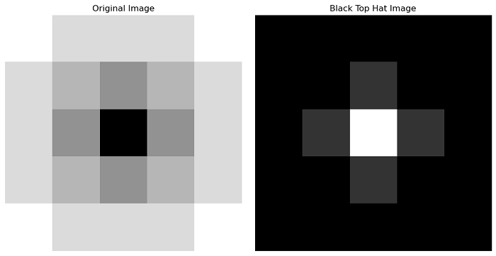
Here's an example of how to use the black_tophat() function.

import numpy as np
import matplotlib.pyplot as plt
from skimage.morphology import black_tophat, square

# Create an example input image
dark_on_gray = np.array([[7, 6, 6, 6, 7],
                         [6, 5, 4, 5, 6],
                         [6, 4, 0, 4, 6],
                         [6, 5, 4, 5, 6],
                         [7, 6, 6, 6, 7]], dtype=np.uint8)

# Apply black top hat using a square-shaped structuring element of size 3x3
result = black_tophat(dark_on_gray, square(3))

# Create subplots to display the original and black top hat images side by side
fig, axes = plt.subplots(1, 2, figsize=(10, 5))
ax = axes.ravel()
ax[0].imshow(dark_on_gray, cmap=plt.cm.gray)
ax[0].set_title('Original Image')
ax[0].set_axis_off()
ax[1].imshow(result, cmap=plt.cm.gray)
ax[1].set_title('Black Top Hat Image')
ax[1].set_axis_off()
plt.tight_layout()
plt.show()

Output

On executing the above program, you will get the following output −