- Scikit Image – Introduction
- Scikit Image - Image Processing
- Scikit Image - Numpy Images
- Scikit Image - Image datatypes
- Scikit Image - Using Plugins
- Scikit Image - Image Handlings
- Scikit Image - Reading Images
- Scikit Image - Writing Images
- Scikit Image - Displaying Images
- Scikit Image - Image Collections
- Scikit Image - Image Stack
- Scikit Image - Multi Image
- Scikit Image - Data Visualization
- Scikit Image - Using Matplotlib
- Scikit Image - Using Ploty
- Scikit Image - Using Mayavi
- Scikit Image - Using Napari
- Scikit Image - Color Manipulation
- Scikit Image - Alpha Channel
- Scikit Image - Conversion b/w Color & Gray Values
- Scikit Image - Conversion b/w RGB & HSV
- Scikit Image - Conversion to CIE-LAB Color Space
- Scikit Image - Conversion from CIE-LAB Color Space
- Scikit Image - Conversion to luv Color Space
- Scikit Image - Conversion from luv Color Space
- Scikit Image - Image Inversion
- Scikit Image - Painting Images with Labels
- Scikit Image - Contrast & Exposure
- Scikit Image - Contrast
- Scikit Image - Contrast enhancement
- Scikit Image - Exposure
- Scikit Image - Histogram Matching
- Scikit Image - Histogram Equalization
- Scikit Image - Local Histogram Equalization
- Scikit Image - Tinting gray-scale images
- Scikit Image - Image Transformation
- Scikit Image - Scaling an image
- Scikit Image - Rotating an Image
- Scikit Image - Warping an Image
- Scikit Image - Affine Transform
- Scikit Image - Piecewise Affine Transform
- Scikit Image - ProjectiveTransform
- Scikit Image - EuclideanTransform
- Scikit Image - Radon Transform
- Scikit Image - Line Hough Transform
- Scikit Image - Probabilistic Hough Transform
- Scikit Image - Circular Hough Transforms
- Scikit Image - Elliptical Hough Transforms
- Scikit Image - Polynomial Transform
- Scikit Image - Image Pyramids
- Scikit Image - Pyramid Gaussian Transform
- Scikit Image - Pyramid Laplacian Transform
- Scikit Image - Swirl Transform
- Scikit Image - Morphological Operations
- Scikit Image - Erosion
- Scikit Image - Dilation
- Scikit Image - Black & White Tophat Morphologies
- Scikit Image - Convex Hull
- Scikit Image - Generating footprints
- Scikit Image - Isotopic Dilation & Erosion
- Scikit Image - Isotopic Closing & Opening of an Image
- Scikit Image - Skelitonizing an Image
- Scikit Image - Morphological Thinning
- Scikit Image - Masking an image
- Scikit Image - Area Closing & Opening of an Image
- Scikit Image - Diameter Closing & Opening of an Image
- Scikit Image - Morphological reconstruction of an Image
- Scikit Image - Finding local Maxima
- Scikit Image - Finding local Minima
- Scikit Image - Removing Small Holes from an Image
- Scikit Image - Removing Small Objects from an Image
- Scikit Image - Filters
- Scikit Image - Image Filters
- Scikit Image - Median Filter
- Scikit Image - Mean Filters
- Scikit Image - Morphological gray-level Filters
- Scikit Image - Gabor Filter
- Scikit Image - Gaussian Filter
- Scikit Image - Butterworth Filter
- Scikit Image - Frangi Filter
- Scikit Image - Hessian Filter
- Scikit Image - Meijering Neuriteness Filter
- Scikit Image - Sato Filter
- Scikit Image - Sobel Filter
- Scikit Image - Farid Filter
- Scikit Image - Scharr Filter
- Scikit Image - Unsharp Mask Filter
- Scikit Image - Roberts Cross Operator
- Scikit Image - Lapalace Operator
- Scikit Image - Window Functions With Images
- Scikit Image - Thresholding
- Scikit Image - Applying Threshold
- Scikit Image - Otsu Thresholding
- Scikit Image - Local thresholding
- Scikit Image - Hysteresis Thresholding
- Scikit Image - Li thresholding
- Scikit Image - Multi-Otsu Thresholding
- Scikit Image - Niblack and Sauvola Thresholding
- Scikit Image - Restoring Images
- Scikit Image - Rolling-ball Algorithm
- Scikit Image - Denoising an Image
- Scikit Image - Wavelet Denoising
- Scikit Image - Non-local means denoising for preserving textures
- Scikit Image - Calibrating Denoisers Using J-Invariance
- Scikit Image - Total Variation Denoising
- Scikit Image - Shift-invariant wavelet denoising
- Scikit Image - Image Deconvolution
- Scikit Image - Richardson-Lucy Deconvolution
- Scikit Image - Recover the original from a wrapped phase image
- Scikit Image - Image Inpainting
- Scikit Image - Registering Images
- Scikit Image - Image Registration
- Scikit Image - Masked Normalized Cross-Correlation
- Scikit Image - Registration using optical flow
- Scikit Image - Assemble images with simple image stitching
- Scikit Image - Registration using Polar and Log-Polar
- Scikit Image - Feature Detection
- Scikit Image - Dense DAISY Feature Description
- Scikit Image - Histogram of Oriented Gradients
- Scikit Image - Template Matching
- Scikit Image - CENSURE Feature Detector
- Scikit Image - BRIEF Binary Descriptor
- Scikit Image - SIFT Feature Detector and Descriptor Extractor
- Scikit Image - GLCM Texture Features
- Scikit Image - Shape Index
- Scikit Image - Sliding Window Histogram
- Scikit Image - Finding Contour
- Scikit Image - Texture Classification Using Local Binary Pattern
- Scikit Image - Texture Classification Using Multi-Block Local Binary Pattern
- Scikit Image - Active Contour Model
- Scikit Image - Canny Edge Detection
- Scikit Image - Marching Cubes
- Scikit Image - Foerstner Corner Detection
- Scikit Image - Harris Corner Detection
- Scikit Image - Extracting FAST Corners
- Scikit Image - Shi-Tomasi Corner Detection
- Scikit Image - Haar Like Feature Detection
- Scikit Image - Haar Feature detection of coordinates
- Scikit Image - Hessian matrix
- Scikit Image - ORB feature Detection
- Scikit Image - Additional Concepts
- Scikit Image - Render text onto an image
- Scikit Image - Face detection using a cascade classifier
- Scikit Image - Face classification using Haar-like feature descriptor
- Scikit Image - Visual image comparison
- Scikit Image - Exploring Region Properties With Pandas
Scikit Image - Finding Local Minima
In image processing, the term "minima" or "minimum" refers to points or regions within a digital image where the pixel values reach their lowest level within a specific neighbourhood. In contrast, finding maxima in an image involves identifying points or regions where the values are at their lowest within a local neighbourhood. Local minima denote notable troughs or regions of low intensity within the data. Finding minima plays a significant role in various image analysis tasks, including feature identification, object segmentation, and image enhancement.
Scikit-image libraries offer functions like local_minima() and h_minima() to detect the local minima within an image.
Using the skimage.morphology.local_minima() function
The local_minima() function is used to identify and locate local minima within an n-dimensional array(image). Local minima are points or regions where the pixel values are at their lowest compared to their neighbouring pixels within a specified neighbourhood.
Syntax
Following is the syntax of this function −
skimage.morphology.local_minima(image, footprint=None, connectivity=None, indices=False, allow_borders=True)
Parameters
- image (ndarray): This is the n-dimensional array on which local minima will find.
- footprint (ndarray, optional): The footprint, also known as the structuring element, is used to determine the neighborhood of each evaluated pixel. It must be a boolean array and have the same number of dimensions as the image. If neither footprint nor connectivity are given, all adjacent pixels are considered part of the neighborhood.
- connectivity (int, optional): This parameter is used to determine the neighborhood of each evaluated pixel. It specifies which adjacent pixels are considered neighbors based on their squared distance from the center. Pixels whose squared distance is less than or equal to connectivity are considered neighbors. This parameter is ignored if the footprint is not None.
- indices (bool, optional): If True, the output will be a tuple of one-dimensional arrays representing the indices (coordinates) of local minima in each dimension. If False, the output will be a boolean array with the same shape as the image, where True indicates the position of local minima, and False indicates other positions.
- allow_borders (bool, optional): If True, it allows plateaus that touch the image border to be considered as valid minima. If set to False, minima that are on the image borders are not considered.
Return Value
It returns minima, which can be either an ndarray or a tuple of ndarrays, depending on the value of the indices parameter.
Example
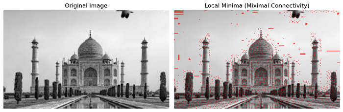
The following example demonstrates how to find and visualize local minima in an image using the local_minima() function.
import numpy as np
from skimage.morphology import local_minima
from skimage.measure import label
import matplotlib.pyplot as plt
from skimage import io, color, exposure

# Load the input image
image = io.imread('Images/Tajmahal.jpg')

# For illustration purposes, we focus on a specific region of the image.
x_0 = 170
y_0 = 100
width = 250
height = 150

# Crop the image to the specified region
image = color.rgb2gray(image)[y_0:(y_0 + height), x_0:(x_0 + width)]

# Rescale the image intensity for visualization purposes.
image = exposure.rescale_intensity(image)

# Find local minima by comparing to all neighboring pixels
minima = local_minima(image)

# Label the local minima to distinguish them
label_minima = label(minima)

# Overlay the labeled local minima on the original image
overlay = color.label2rgb(label_minima, image, alpha=0.7, bg_label=0, bg_color=None, colors=[(1, 0, 0)])

# Plot the original and the resultant images
fig, axes = plt.subplots(1, 2, figsize=(10, 5))
ax = axes.ravel()

# Display the original image
ax[0].imshow(image, cmap=plt.cm.gray)
ax[0].axis('off')
ax[0].set_title('Original Image)

# Display the local minima
ax[1].imshow(overlay, cmap=plt.cm.gray)
ax[1].axis('off')
ax[1].set_title('Local Minima (Miximal Connectivity)')

plt.tight_layout()
plt.show()
Output
On executing the above program, you will get the following output −
Using the skimage.morphology.h_minima() function
The h_minima() function is used to find all minima in an image with a minimum depth condition. These local minima are defined as connected sets of pixels with equal gray levels that are strictly smaller than the gray levels of all neighboring pixels.
A local minimum with a depth of 'h' is a point where there exists a path connecting it to another local minimum with the same or lower value. Along this path, the highest value does not exceed 'f(M) + h' compared to the starting minimum's value. Additionally, there should be no path to any other local minimum with an equal or lower value where the highest value is smaller than 'f(M) + h.' This function also identifies the global minima within the image.
Syntax
Following is the syntax of this function −
skimage.morphology.h_minima(image, h, footprint=None)
Parameters
- image (ndarray): This is the input image on which minima will be found.
- h (unsigned integer): The minimal depth of all extracted minima.
- footprint (ndarray, optional): The neighborhood expressed as an n-dimensional array of 1s and 0s. The default is a neighborhood defined as a ball of radius 1 according to the maximum norm. In 2D, this corresponds to a 3x3 square.
Return Value
It returns h_min, which is an ndarray representing the local minima of depth greater than or equal to h, including the global maxima. The resulting image is binary, where pixels belonging to the determined minima are set to 1, and others are set to 0.
Example
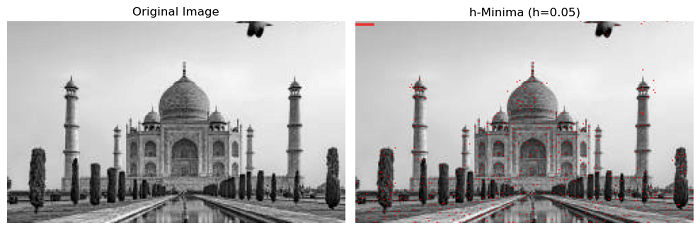
The following example demonstrates how to find the h-minima of an image using the h_minima() function.
import numpy as np
from skimage.morphology import h_minima  # Corrected import
from skimage.measure import label
import matplotlib.pyplot as plt
from skimage import io, color, exposure

# Load the input image
image = io.imread('Images/Tajmahal.jpg')

# For illustration purposes, we focus on a specific region of the image
x_0 = 170
y_0 = 100
width = 250
height = 150

# Crop the image to the specified region
image = color.rgb2gray(image[y_0:(y_0 + height), x_0:(x_0 + width)])

# Rescale the intensity of the image for better visualization
image = exposure.rescale_intensity(image)

# Set the h parameter for h_minima
h = 0.05

# Find h-minima in the cropped and rescaled image
h_minima_image = h_minima(image, h)

# Label the h-minima to distinguish them
labeled_h_minima = label(h_minima_image)

# Overlay the labeled h-minima on the original image
overlay = color.label2rgb(labeled_h_minima, image, alpha=0.7, bg_label=0, bg_color=None, colors=[(1, 0, 0)])

# Create subplots for displaying the original image and h-minima
fig, axes = plt.subplots(1, 2, figsize=(10, 5))
ax = axes.ravel()

# Display the original image
ax[0].imshow(image, cmap=plt.cm.gray)
ax[0].axis('off')
ax[0].set_title('Original Image')

# Display the h-minima overlay
ax[1].imshow(overlay, cmap=plt.cm.gray)
ax[1].axis('off')
ax[1].set_title('h-Minima (h={})'.format(h))

plt.tight_layout()
plt.show()
Output
On executing the above program, you will get the following output −