Scikit Image - Haar Feature Detection of Coordinates

Quiz

Haar feature detection, also known as Haar-like feature detection, is a technique used in computer vision and object recognition to identify specific patterns or objects within an image.

The coordinates of Haar-like features detection refer to the positions within an image where Haar-like features are computed. These coordinates specify where the analysis of pixel intensity differences occurs to identify specific patterns or objects.

The scikit-image library offers the haar_like_feature_coord() function within its feature module to compute the coordinates of Haar-like features within a detection window.

Using the skimage.feature.haar_like_feature_coord()

The haar_like_feature_coord() function is used to compute the coordinates of Haar-like features based on the specified parameters.

Syntax

Here is the syntax of this function −

skimage.feature.haar_like_feature_coord(width, height, feature_type=None)

Parameters

Here is an explanation of its parameters −

width (int): Width of the detection window.
height (int): Height of the detection window.
feature_type (str or list of str or None, optional): Specifies the type of Haar-like feature to consider. It can be one of the following types −
- 'type-2-x': 2 rectangles varying along the x-axis.
- 'type-2-y': 2 rectangles varying along the y-axis.
- 'type-3-x': 3 rectangles varying along the x-axis.
- 'type-3-y': 3 rectangles varying along the y-axis.
'type-4': 4 rectangles varying along both x and y axes.

By default, all available features are extracted. You can provide a list of feature types if you want to compute specific types of Haar-like features.

The function returns two ndarrays −

feature_coord (n_features, n_rectangles, 2, 2), ndarray of list of tuple: This is a NumPy array containing the coordinates of the rectangles for each feature.
feature_type (n_features,), ndarray of str: This array contains the corresponding type for each feature, as specified in the feature_type parameter.

Example

The following example demonstrates how to use the haar_like_feature_coord() function to generate Haar-like feature coordinates and types for a specified window size and feature type.

import numpy as np
from skimage.feature import haar_like_feature_coord

# Define the size of the Haar-like feature window
width, height = 2, 2

# Choose a specific Haar-like feature type (you've already chosen 'type-4')
feat_coord, feat_type = haar_like_feature_coord(width, height, 'type-4')

print("Haar-like feature coordinates:")
print(feat_coord)

print("Haar-like feature types:")
print(feat_type)

Output

Haar-like feature coordinates:
[list([[(0, 0), (0, 0)], [(0, 1), (0, 1)], [(1, 1), (1, 1)], [(1, 0), (1, 0)]])]

Haar-like feature types:
['type-4']

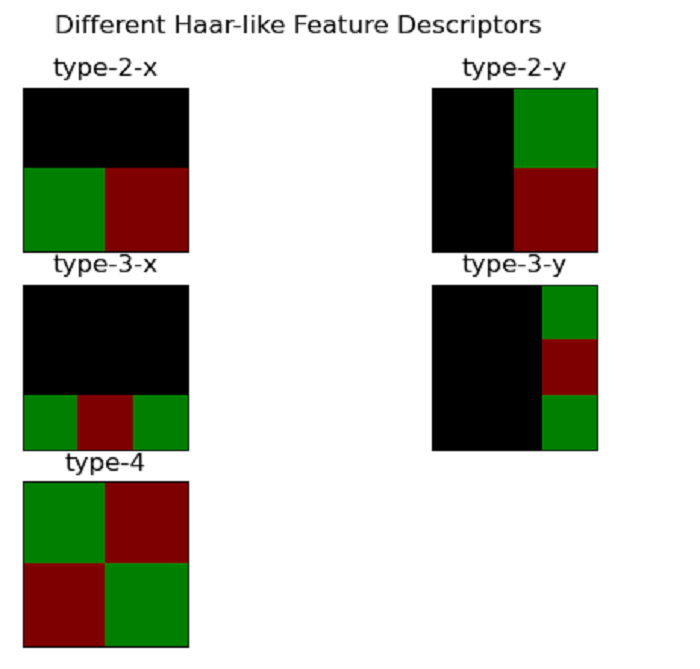
Different types of Haar-like feature descriptors

There are five distinct types of Haar-like feature descriptors, as illustrated using the below example. The descriptor's value corresponds to the contrast between the sum of intensity values in the green and red regions.

Example

The following example generates and displays different Haar-like feature descriptors for various types and different sizes of binary images using the haar_like_feature_coord() and draw_haar_like_feature() functions. Each subplot in the resulting figure represents a different Haar-like feature type applied to a specific image size.

import numpy as np
import matplotlib.pyplot as plt
from skimage.feature import haar_like_feature_coord, draw_haar_like_feature

# Create a list of example images and Haar-like feature types
images = [np.zeros((2, 2)), np.zeros((2, 2)),
   np.zeros((3, 3)), np.zeros((3, 3)),
   np.zeros((2, 2))]

feature_types = ['type-2-x', 'type-2-y',
   'type-3-x', 'type-3-y',
   'type-4']

# Create subplots for displaying Haar-like features
fig, axs = plt.subplots(3, 2)

# Iterate through the images and feature types
for ax, img, feat_type in zip(np.ravel(axs), images, feature_types):
    
   # Get Haar-like feature coordinates for the image
   coord, _ = haar_like_feature_coord(img.shape[0], img.shape[1], feat_type)
   
   # Draw and display the Haar-like feature
   haar_feature = draw_haar_like_feature(img, 0, 0, img.shape[0], img.shape[1], coord, max_n_features=1, random_state=0)
   ax.imshow(haar_feature)
   ax.set_title(feat_type)
   ax.set_xticks([])
   ax.set_yticks([])

# Set the title and hide axis labels
fig.suptitle('Different Haar-like Feature Descriptors')
plt.axis('off')
plt.show()

Output

Print Page