Scikit Image - Finding Contour

Quiz

In image processing, a contour is a continuous curve that connects points with the same color or intensity along a boundary. Finding contours play a crucial role in shape analysis and object detection, aiding in the identification and characterization of objects within an image.

The Scikit-Image library offers a powerful tool for finding contours using the find_contours() function within its measure module to find the contours using the marching squares method.

Using the skimage.measure.find_contours() function

The measure.find_contours() function is used to find iso-valued contours in a 2D array for a given level value. It's a useful tool for tasks like identifying boundaries or shapes within an image.

It employs the 'marching squares' technique to calculate iso-valued contours within the input 2D array at a specified level value. To enhance precision in the resulting contours, the array values undergo linear interpolation.

Syntax

Following is the syntax of this function −

skimage.measure.find_contours(image, level=None, fully_connected='low', positive_orientation='low', *, mask=None)

Parameters

Here are the parameters and their explanations −

image (2D ndarray of double): This is the input image in which to find contours.
level (float, optional): This parameter specifies the value along which to find contours in the array. By default, the level is set to the midpoint between the maximum and minimum values in the image (i.e. (max(image) + min(image)) / 2).
fully_connected (str, {'low', 'high'}): This parameter determines whether array elements below the given level value are considered fully connected (and hence elements above the value will only be face connected), or vice versa.
positive_orientation (str, {'low', 'high'}): This parameter indicates whether the output contours will produce positively-oriented polygons around islands of low- or high-valued elements. The options are:
'low': Contours will wind counter-clockwise around elements below the iso-value.
'high': Contours will wind counter-clockwise around elements above the iso-value.
mask (2D ndarray of bool, or None): A boolean mask that indicates where you want to draw contours. If a mask is passed, contours will only be computed in regions where the mask is True. NaN values in the image are automatically excluded from the considered region (the mask is set to False wherever the array is NaN).

The function returns a list of (n,2)-ndarrays, where each contour is an ndarray of shape (n, 2), consisting of n (row, column) coordinates along the contour.

Example

Here is an example that uses the find_contours() function to detect contours within an array at a level of 0.5.

import numpy as np
from skimage.measure import find_contours

# Create a 3x3 NumPy array
a = np.zeros((3, 3))

# Set one element to a value of 1
a[0, 0] = 1

# Display the input array 
print("Input Array:")
print(a)

# Find contours in the array at a level of 0.5
contours = find_contours(a, 0.5)

# Display the contours found
print("Contours:")
for contour in contours:
   print(contour)

Output

Input Array:
[[1. 0. 0.]
 [0. 0. 0.]
 [0. 0. 0.]]

Contours:
[[0.  0.5]
 [0.5 0. ]]

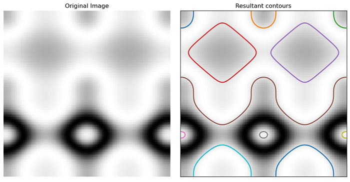
Example

The following example demonstrates the process of finding contours in an image using the skimage.measure.find_contours() function.

import numpy as np
import matplotlib.pyplot as plt
from skimage import measure

# Create some test data
x, y = np.ogrid[-np.pi:np.pi:100j, -np.pi:np.pi:100j]
array = np.sin(np.exp(np.sin(x)**3 + np.cos(y)**2))

# Find contours in 'r' at a constant value of 0.8
contours = measure.find_contours(array, 0.8)

# Create a figure and axes for displaying the image and contours
fig, ax = plt.subplots(1,2, figsize=(10, 5))

# Display the grayscale image
ax[0].imshow(array, cmap=plt.cm.gray)
ax[0].set_title('Original Image')
ax[0].axis('off')

ax[1].imshow(array, cmap=plt.cm.gray)
ax[1].set_title('Resultant contours')

# Plot each contour found with a linewidth of 2
for contour in contours:
   ax[1].plot(contour[:, 1], contour[:, 0], linewidth=2)
    
# Set axis properties for image display
ax[1].axis('image')
ax[1].set_xticks([])
ax[1].set_yticks([])

plt.tight_layout()
plt.show()

Output

Print Page