Scikit Image - Sliding Window Histogram

Quiz

The sliding window algorithm is a fundamental technique in computer vision and image processing, widely employed for localized analysis of images. On the other hand, histogram matching involves comparing the histograms of two images to discover similarities and can be used for object detection in images.

A sliding window histogram is a technique used in image processing to analyze the local distribution of pixel values within an image. It involves moving a small "window" or "kernel" across the image and computing a histogram within that window at each position.

This tutorial extracts a small region from an input image and uses histogram matching to attempt to locate a similar region within the original image.

Computing a sliding window histogram is common in solving computer vision problems such as object detection, object tracking, and image filtering. The scikit-image library provides the filters.rank.windowed_histogram() function for this purpose, as it uses an efficient sliding window-based algorithm that is able to compute these histograms quickly.

Using the skimage.filters.rank.windowed_histogram() function

The skimage.filters.rank.windowed_histogram() function is used to compute the normalized sliding window histogram of an input image. It calculates histograms within local neighborhoods defined by a specified footprint and an optional mask.

Syntax

skimage.filters.rank.windowed_histogram(image, footprint, out=None, mask=None, shift_x=False, shift_y=False, n_bins=None)

Parameters

The function accepts the following parameters −

image (2-D array (integer or float)): Input image on which the windowed histogram will be calculated.
Footprint (2-D array (integer or float)): The neighborhood is expressed as a 2-D array of 1's and 0's.
out (2-D array (integer or float), optional): If provided, it is an output array where the results will be stored. If None, a new array will be allocated for the output.
mask (ndarray (integer or float), optional): A mask array that defines the area of the image included in the local neighborhood. The mask is typically used to restrict histogram calculations to specific regions of interest. If None, the complete image is used as the mask by default.
shift_x, shift_y (int, optional): Offsets added to the footprint center point. The shift is bounded to the footprint sizes, ensuring that the center remains inside the footprint.
n_bins (int or None, optional): The number of histogram bins. If provided, it specifies the number of bins for the histogram. If set to None, the number of bins will default to image.max() + 1.

The function returns an output array out, which is a 3-D array of dimensions (H, W, N), where (H, W) are the dimensions of the input image, and N is the number of histogram bins (n_bins) or image.max() + 1 if no n_bins value is provided. Each pixel in the output array is an N-dimensional feature vector that represents the histogram. The sum of the elements in the feature vector is 1, except when no pixels in the window are covered by both the footprint and the mask, in which case all elements will be 0.

Example

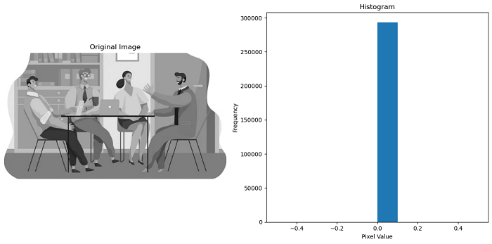
Here is a simple example that calculates the windowed histogram of the input image using the skimage.filters.rank.windowed_histogram() function.

import numpy as np
import matplotlib.pyplot as plt
from skimage import io
from skimage.filters.rank import windowed_histogram
from skimage.morphology import disk

# Load the input image
img = io.imread('Images/group chat.jpg', as_gray=True)

# Calculate the windowed histogram of the camera image
hist_img = windowed_histogram(img, disk(5))

# Create subplots to display the original image and the selected windowed histogram slice
fig, axes = plt.subplots(1, 2, figsize=(12, 6))

# Plot the original image
axes[0].imshow(img, cmap='gray')
axes[0].set_title('Original Image')
axes[0].axis('off')

# Flatten the histogram image and calculate the histogram
hist_values = hist_img.ravel()

# Plot the histogram
axes[1].hist(hist_values)
axes[1].set_title('Histogram')
axes[1].set_xlabel('Pixel Value')
axes[1].set_ylabel('Frequency')

plt.tight_layout()
plt.show()

Output

Example

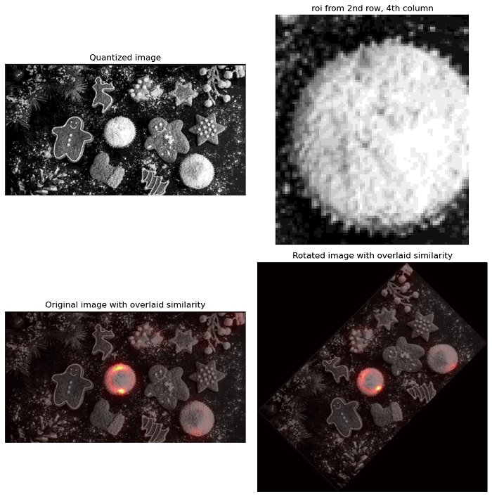
The following example demonstrates the use of the windowed_histogram function to compare a region of interest (ROI) in an image to the within the original image.

import numpy as np
import matplotlib.pyplot as plt
from skimage import io, transform
from skimage.util import img_as_ubyte
from skimage.morphology import disk
from skimage.filters import rank

def windowed_histogram_similarity(image, footprint, reference_hist, n_bins):
   # Compute normalized windowed histogram feature vector for each pixel
   px_histograms = rank.windowed_histogram(image, footprint, n_bins=n_bins)
   
   # Reshape the reference histogram for broadcasting
   reference_hist = reference_hist.reshape((1, 1) + reference_hist.shape)
   
   # Compute Chi squared distance metric: sum((X-Y)^2 / (X+Y))
   X = px_histograms
   Y = reference_hist
   num = (X - Y) ** 2
   denom = X + Y
   denom[denom == 0] = np.inf  # Prevent division by zero
   frac = num / denom
   chi_sqr = 0.5 * np.sum(frac, axis=2)
   
   # Generate a similarity measure, taking the reciprocal
   # to make it higher when distance is low
   similarity = 1 / (chi_sqr + 1.0e-4)
   
   return similarity

# Load the input image and convert it to grayscale
img = img_as_ubyte(io.imread('Images/decore.png', as_gray=True))

# Quantize the image to 16 levels of grayscale
quantized_img = img // 16

# Select a region of interest in the image  
roi = quantized_img[120:215, 240:320]

# Compute roi histogram and normalize it
roi_hist, _ = np.histogram(roi.flatten(), bins=16, range=(0, 16))
roi_hist = roi_hist.astype(float) / np.sum(roi_hist)

# Create a disk-shaped mask for sliding window
footprint = disk(30)

# Compute similarity across the entire image
similarity = windowed_histogram_similarity(quantized_img, footprint, roi_hist,
   roi_hist.shape[0])

# Rotate the image by 45 degrees
rotated_img = img_as_ubyte(transform.rotate(img, 45.0, resize=True))
quantized_rotated_image = rotated_img // 16

# Compute similarity on the rotated image
rotated_similarity = windowed_histogram_similarity(quantized_rotated_image,
   footprint, roi_hist,
   roi_hist.shape[0])

# Create subplots to display results
fig, axes = plt.subplots(nrows=2, ncols=2, figsize=(10, 10))

axes[0, 0].imshow(quantized_img, cmap='gray')
axes[0, 0].set_title('Quantized image')
axes[0, 0].axis('off')

axes[0, 1].imshow(roi, cmap='gray')
axes[0, 1].set_title('roi from 2nd row, 4th column')
axes[0, 1].axis('off')

axes[1, 0].imshow(img, cmap='gray')
axes[1, 0].imshow(similarity, cmap='hot', alpha=0.5)
axes[1, 0].set_title('Original image with overlaid similarity')
axes[1, 0].axis('off')

axes[1, 1].imshow(rotated_img, cmap='gray')
axes[1, 1].imshow(rotated_similarity, cmap='hot', alpha=0.5)
axes[1, 1].set_title('Rotated image with overlaid similarity')
axes[1, 1].axis('off')

plt.tight_layout()
plt.show()

Output

Print Page