Recover the Original from a Wrapped Phase Image

---

---

The process of recovering the original from a wrapped phase image typically involves a technique called "phase unwrapping. The phase unwrapping method aims to retrieve the underlying, continuous, or unwrapped phase information from an image or signal that has undergone a wrapping process.

In some situations, certain signals or images are restricted to values within a limited range (modulo 2*pi). In these cases, phase unwrapping is used to recover the underlying, unwrapped signal. In this tutorial, we'll see about the scikit-image (skimage) provided phase unwrapping algorithm on one-dimensional, two-dimensional, and three-dimensional images.

Using the skimage.restoration.unwrap_phase() function

The restoration.unwrap_phase() function is used to recover the original, unwrapped image from a wrapped phase image. It recovers an image from a wrapped image having values that lie in the interval [-pi, pi), and recovers the original, unwrapped image.

Syntax

Following is the syntax of this function −

skimage.restoration.unwrap_phase(image, wrap_around=False, rng=None)

Parameters

Here are the details about the function parameters −

• image: This is a 1D, 2D, or 3D ndarray of floats, optionally a masked array. It represents the wrapped phase image and values in this image should be in the range [-pi, pi). If a masked array is provided, the masked entries will not be changed, and their values will not be used to guide the unwrapping of neighboring, unmasked values. However, masked 1D arrays are not allowed and will raise a ValueError.

• wrap_around (optional): This parameter is a boolean or a sequence of booleans. When an element of the sequence is True, the unwrapping process will regard the edges along the corresponding axis of the image to be connected and use this connectivity to guide the phase unwrapping process. If only a single boolean is given, it will apply to all axes. This wrap-around is not supported for 1D arrays.

• rng (optional): This parameter specifies the pseudo-random number generator used for initialization during the unwrapping process. By default, a PCG64 generator is used (see numpy.random.default_rng()). If rng is an integer, it is used to seed the generator. Setting a specific seed can be useful for achieving deterministic behavior in the unwrapping process.

The function returns an unwrapped image (image_unwrapped: array_like, double) of the same shape as the input. If the input image is a masked array, the mask information will be preserved in the output.

Additionally, the function can raise a ValueError in the following cases −

• If called with a masked 1D array.

• If called with a 1D array and wrap_around=True.

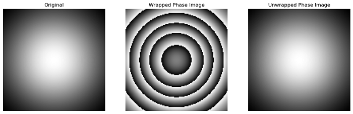
Example

The following example demonstrates how to use the unwrap_phase() function to unwrap a wrapped phase image.

import numpy as np
import matplotlib.pyplot as plt
from skimage.restoration import unwrap_phase

# Create the coordinate grids
c0, c1 = np.ogrid[-1:1:128j, -1:1:128j]

# Create the input wrapped phase image
image = 12 * np.pi * np.exp(-(c0**2 + c1**2))
image_wrapped = np.angle(np.exp(1j * image))

# Unwrap the phase image
image_unwrapped = unwrap_phase(image_wrapped)

# Create subplots for the display the results 
fig, axes = plt.subplots(1, 3, figsize=(15, 5))
ax = axes.ravel()
plt.gray()

# Display the original image
ax[0].imshow(image)
ax[0].set_title('Original')
ax[0].axis('off')

# Display the Wrapped Phase Image
ax[1].imshow(image_wrapped)
ax[1].set_title('Wrapped Phase Image')
ax[1].axis('off')

# Unwrapped Phase Image
ax[2].imshow(image_unwrapped)
ax[2].set_title('Unwrapped Phase Image')
ax[2].axis('off')
    
plt.show()

Output

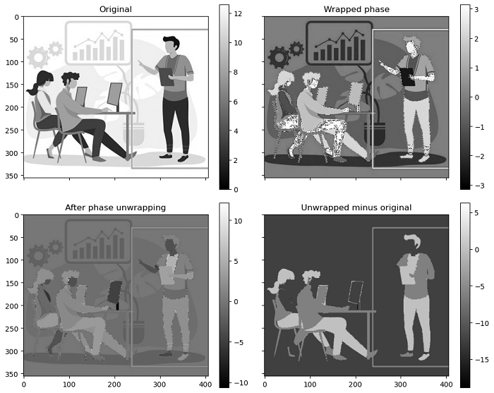
Example

The following example demonstrates the process of phase unwrapping using the unwrap_phase() function of a two dimensional wrapped phase image.

import numpy as np
import matplotlib.pyplot as plt
from skimage import color, io, exposure
from skimage.restoration import unwrap_phase

# Load an image as a floating-point grayscale
original_image = color.rgb2gray(io.imread('Images/image5.jpg'))

# Scale the image to the range [0, 4*pi]
scaled_image = exposure.rescale_intensity(original_image, out_range=(0, 4 * np.pi))

# Create a phase-wrapped image in the interval [-pi, pi)
wrapped_phase_image = np.angle(np.exp(1j * scaled_image))

# Perform phase unwrapping
unwrapped_phase_image = unwrap_phase(wrapped_phase_image)

# Create subplots for visualization
fig, axes = plt.subplots(2, 2, sharex=True, sharey=True)
ax1, ax2, ax3, ax4 = axes.ravel()

# Display the original image
ax1.imshow(scaled_image, cmap='gray', vmin=0, vmax=4 * np.pi)
ax1.set_title('Original')

# Display the wrapped phase image
ax2.imshow(wrapped_phase_image, cmap='gray', vmin=-np.pi, vmax=np.pi)
ax2.set_title('Wrapped phase')

# Display the unwrapped phase image
ax3.imshow(unwrapped_phase_image, cmap='gray')
ax3.set_title('After phase unwrapping')

# Display the difference between unwrapped and original
ax4.imshow(unwrapped_phase_image - scaled_image, cmap='gray')
ax4.set_title('Unwrapped minus original')

# Add colorbars for reference
for ax in axes.ravel():
   fig.colorbar(ax.get_images()[0], ax=ax)

plt.tight_layout()
plt.show()

Output

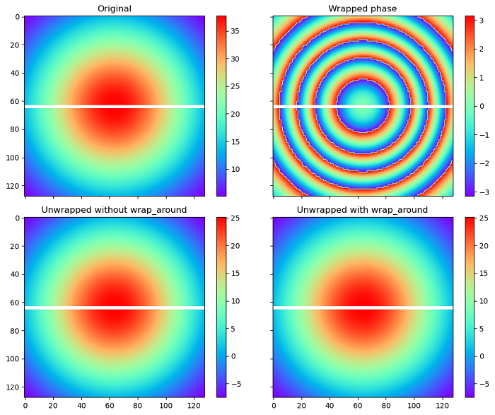
Unwrapping with Masked Arrays

The unwrapping procedure (unwrap_phase() function) can accept masked arrays as input. When a masked array is provided, the values in the masked entries are not changed during the unwrapping process. Additionally, the values of masked entries are not used to guide the unwrapping of neighboring unmasked values.

Example

Here is an example that demonstrates the unwrapping of the wrapped phase image with a mask using the unwrap_phase() function with and without wrap-around enabled.

import numpy as np
import matplotlib.pyplot as plt
from skimage.restoration import unwrap_phase

# Create the coordinate grids
c0, c1 = np.ogrid[-1:1:128j, -1:1:128j]

# Create the input image
image = 12 * np.pi * np.exp(-(c0**2 + c1**2))

# Mask the image to split it in two horizontally
mask = np.zeros_like(image, dtype=bool)
mask[image.shape[0] // 2, :] = True

# Compute the wrapped phase image
image_wrapped = np.ma.array(np.angle(np.exp(1j * image)), mask=mask)

# Unwrap image without wrap around
image_unwrapped_no_wrap_around = unwrap_phase(image_wrapped, wrap_around=(False, False))

# Unwrap with wrap around enabled for the 0th dimension
image_unwrapped_wrap_around = unwrap_phase(image_wrapped, wrap_around=(True, False))

# Create subplots for visualization
fig, ax = plt.subplots(2, 2, figsize=(10, 8),sharex=True, sharey=True)
ax1, ax2, ax3, ax4 = ax.ravel()

# Plot the original image with the mask
fig.colorbar(ax1.imshow(np.ma.array(image, mask=mask), cmap='rainbow'), ax=ax1)
ax1.set_title('Original')

# Plot the wrapped phase image
fig.colorbar(ax2.imshow(image_wrapped, cmap='rainbow', vmin=-np.pi, vmax=np.pi), ax=ax2)
ax2.set_title('Wrapped phase')

# Plot the unwrapped image without wrap_around
fig.colorbar(ax3.imshow(image_unwrapped_no_wrap_around, cmap='rainbow'), ax=ax3)
ax3.set_title('Unwrapped without wrap_around')

# Plot the unwrapped image with wrap_around
fig.colorbar(ax4.imshow(image_unwrapped_wrap_around, cmap='rainbow'), ax=ax4)
ax4.set_title('Unwrapped with wrap_around')

plt.tight_layout()
plt.show()

Output