Scikit Image - Extracting FAST Corners

Quiz

FAST (Features from Accelerated Segment Test) is a corner detection method widely employed for feature point extraction, particularly in the context of computer vision applications like object tracking and mapping. It was originally developed by Edward Rosten and Tom Drummond in 2006, and offers a significant advantage in terms of computational speed. As its name suggests it is indeed faster than many other well-known feature extraction methods, including the Difference of Gaussians (DoG) utilized by SIFT, SUSAN, and Harris detectors.

The FAST corner detector relies on a circle of 16 pixels, equivalent to a Bresenham circle with a radius of 3, to determine whether a candidate point 'p' qualifies as a corner. Each pixel around the circle is assigned an integer label from 1 to 16, in clockwise order. 'p' is considered a corner if a continuous set of 'N' neighboring pixels in the circle are all either brighter than 'p' by a threshold value 't' or darker than 'p' by 't'. This method efficiently identifies corners in images.

The scikit image library offers the corner_fast function within its feature module to extract the extract feature points from an image.

Using the skimage.feature.corner_fast() function

The corner_fast() function is used for extracting FAST corners from an image.

Syntax

Here is the syntax of the function −

skimage.feature.corner_fast(image, n=12, threshold=0.15)

Parameters

Here are the details of its parameters −

image (M, N) ndarray: The input image from which FAST corners will be extracted.
n (int, optional): This parameter specifies the minimum number of consecutive pixels out of 16 pixels on a circle that should all be either brighter or darker w.r.t testpixel. In other words, it controls the threshold for classifying a point c on the circle as darker (if Ic < Ip - threshold) or brighter (if Ic > Ip + threshold) relative to the test pixel p. Additionally, it represents the 'n' in the FAST-n corner detector.
threshold (float, optional): The threshold used to determine whether the pixels on the circle are brighter, darker, or similar to the test pixel. Decreasing the threshold tends to yield more corners while increasing it results in fewer detected corners.

The function returns the response (ndarray) represents the FAST corner response image.

Example

Here is an example that demonstrates how to use the FAST corner detection method using the corner_fast() function from the scikit-image library to extract the FAST corners in a simple 12x12 array.

from skimage.feature import corner_fast, corner_peaks
import numpy as np

# Create a 12x12 array with a square-shaped region
square = np.zeros((12, 12))
square[3:9, 3:9] = 1
square.astype(int)

# Display the input array
print("Input array:")
print(square)

# Extract Fast corners
corners = corner_fast(square, 9)

# Use corner_peaks to find corner coordinates with a minimum distance of 1 pixel
coords = corner_peaks(corners, min_distance=1)

# Display the corner coordinates
print("Corner Coordinates:")
print(coords)

Output

Input array:
[[0. 0. 0. 0. 0. 0. 0. 0. 0. 0. 0. 0.]
 [0. 0. 0. 0. 0. 0. 0. 0. 0. 0. 0. 0.]
 [0. 0. 0. 0. 0. 0. 0. 0. 0. 0. 0. 0.]
 [0. 0. 0. 1. 1. 1. 1. 1. 1. 0. 0. 0.]
 [0. 0. 0. 1. 1. 1. 1. 1. 1. 0. 0. 0.]
 [0. 0. 0. 1. 1. 1. 1. 1. 1. 0. 0. 0.]
 [0. 0. 0. 1. 1. 1. 1. 1. 1. 0. 0. 0.]
 [0. 0. 0. 1. 1. 1. 1. 1. 1. 0. 0. 0.]
 [0. 0. 0. 1. 1. 1. 1. 1. 1. 0. 0. 0.]
 [0. 0. 0. 0. 0. 0. 0. 0. 0. 0. 0. 0.]
 [0. 0. 0. 0. 0. 0. 0. 0. 0. 0. 0. 0.]
 [0. 0. 0. 0. 0. 0. 0. 0. 0. 0. 0. 0.]]

Corner Coordinates:
[[3 3]
 [3 8]
 [8 3]
 [8 8]]

Example

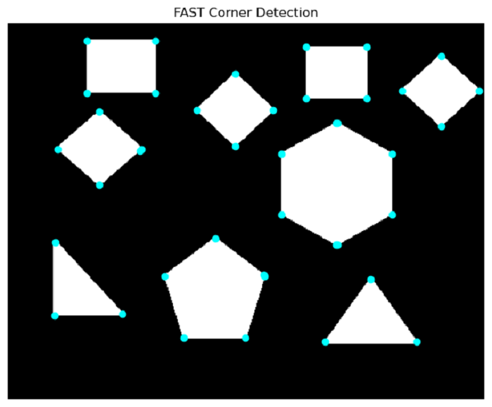
This example demonstrates how to apply the FAST corner detection algorithm to an image using the corner_fast() function.

from skimage.feature import corner_fast, corner_peaks
from skimage import io
import matplotlib.pyplot as plt

# Load an image
image = io.imread('Images/sample.png', as_gray=True)

# Apply corner_fast to detect FAST corners
fast_corners = corner_fast(image, n=9, threshold=0.15)

# Use corner_peaks to find corner coordinates with a minimum distance of 1 pixel
coords = corner_peaks(fast_corners, min_distance=1)

# Create a plot to display the image and detected corners
plt.figure(figsize=(8, 8))
plt.imshow(image, cmap='gray')

# Mark the detected corners with red dots
plt.plot(coords[:, 1], coords[:, 0], color='cyan', marker='o', linestyle='None', markersize=6)

plt.title('FAST Corner Detection')
plt.axis('off')
plt.show()

Output

Print Page