Scikit Image - Active Contour Model

Quiz

The active contour model, also known as the snake model, is a widely used technique in image processing and computer vision. It was introduced by Michael Kass, Andrew Witkin, and Demetri Terzopoulos for contour extraction and object boundary detection.

This model operates by fitting open or closed splines to lines or edges present within an image. The process involves minimizing an energy function that combines information from both the image and the spline's shape, including its length and smoothness. The minimization is performed implicitly in the shape energy and explicitly in the image energy.

The scikit-image library offers the active_contour function within its segmentation submodule to apply the active contour model.

Using the skimage.segmentation.active_contour() function

The segmentation.active_contour() function is used for the active contour model. Active contours by fitting snakes to features of images, allowing for segmentation and boundary detection. This function supports both single and multichannel 2D images and provides flexibility for configuring the behavior of the snake.

Syntax

Following is the syntax of this function −

skimage.segmentation.active_contour(image, snake, alpha=0.01, beta=0.1, w_line=0, w_edge=1, gamma=0.01, max_px_move=1.0, max_num_iter=2500, convergence=0.1, *, boundary_condition='periodic')

Parameters

The function accepts the following parameters −

image: (N, M) or (N, M, 3) ndarray: This parameter represents the input image.
snake: (N, 2) ndarray : This parameter specifies the initial snake coordinates. For periodic boundary conditions, ensure that the endpoints are not duplicated.
alpha: float, optional : Snake length shape parameter. Higher values make the snake contract faster.
beta: float, optional : Snake smoothness shape parameter. Higher values result in a smoother snake.
w_line: float, optional : Controls attraction to brightness. Use negative values to attract the snake toward dark regions.
w_edge: float, optional : Controls attraction to edges. Use negative values to repel the snake from edges.
gamma: float, optional : Explicit time stepping parameter.
max_px_move: float, optional : Specifies the maximum pixel distance the snake can move per iteration.
max_num_iter: int, optional : Sets the maximum number of iterations to optimize the snake's shape.
convergence: float, optional : Convergence criteria.
boundary_condition: string, optional : Defines the boundary conditions for the contour. It can take one of the following values: 'periodic', 'free', 'fixed', 'free-fixed', or 'fixed-free'. 'periodic' attach the two ends of the snake, 'fixed' holds the end-points in place, and 'free' allows free movement of the ends. 'fixed' and 'free' can be combined by parsing 'fixed-free' or 'free-fixed'. Parsing 'fixed-fixed' or 'free-free' yields the same behavior as 'fixed' and 'free', respectively.

The function returns the optimized snake((N, 2) ndarray), which has the same shape as the input parameter.

Example

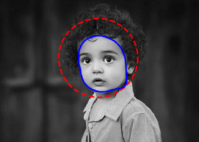
In the following two examples, the active contour model is used to segment the face of a person from the rest of an image by fitting a closed curve to the edges of the face using the active_contour() function.

import numpy as np
import matplotlib.pyplot as plt
from skimage.color import rgb2gray
from skimage import io
from skimage.filters import gaussian
from skimage.segmentation import active_contour

# Load the input image as a grayscale image
img = io.imread('Images/boy.jpg', as_gray=True)

# Create initial snake coordinates
s = np.linspace(0, 2*np.pi, 400)
r = 150 + 100*np.sin(s)
c = 250 + 100*np.cos(s)
init = np.array([r, c]).T

# Apply the active contour model to segment the image
snake = active_contour(gaussian(img, sigma=3, preserve_range=False),
   init, alpha=0.015, beta=10, gamma=0.001)

# Create a plot to visualize the original image and the snake
fig, ax = plt.subplots(figsize=(7, 7))
ax.imshow(img, cmap=plt.cm.gray)
ax.plot(init[:, 1], init[:, 0], '--r', lw=3)  
ax.plot(snake[:, 1], snake[:, 0], '-b', lw=3) 
ax.set_xticks([]), ax.set_yticks([])  
ax.axis([0, img.shape[1], img.shape[0], 0])  

plt.show()

Output

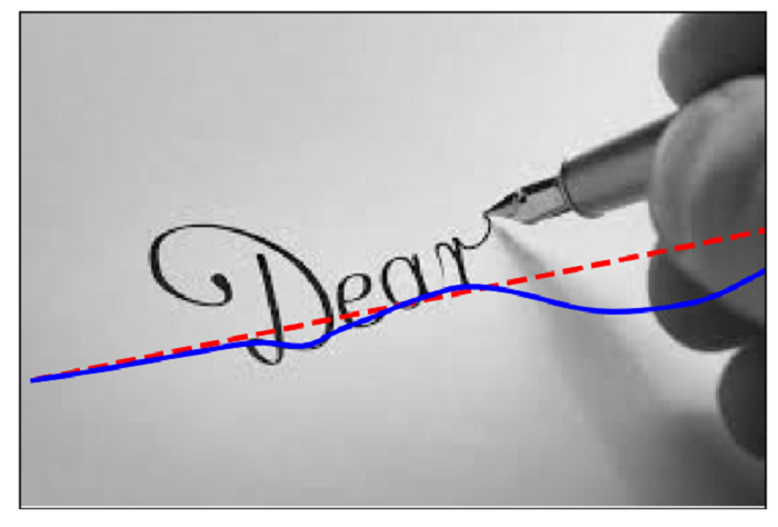
Example

In this example, the active contour model is used to find the darkest curve between two fixed points while obeying smoothness considerations. It initializes a straight line between the two fixed points, (5, 136) and (424, 50), and ensures that the spline's endpoints remain fixed by specifying the boundary condition as boundary_condition='fixed'. Additionally, the algorithm is instructed to search for dark lines by assigning a negative value to w_line.

import numpy as np
import matplotlib.pyplot as plt
from skimage.color import rgb2gray
from skimage import io
from skimage.filters import gaussian
from skimage.segmentation import active_contour

# Load the input image
img = io.imread('Images/hand writting.jpg', as_gray=True)

# Create initial snake coordinates
r = np.linspace(136, 50, 100)
c = np.linspace(5, 424, 100)
init = np.array([r, c]).T

# Apply the active contour model to segment the text in the image
snake = active_contour(gaussian(img, sigma=1, preserve_range=False),
   init, boundary_condition='fixed',
   alpha=0.1, beta=1.0, w_line=-5, w_edge=0, gamma=0.1)

# Create a plot to visualize the original image and the snake
fig, ax = plt.subplots(figsize=(9, 5))
ax.imshow(img, cmap=plt.cm.gray)
ax.plot(init[:, 1], init[:, 0], '--r', lw=3)  # Initial snake in red
ax.plot(snake[:, 1], snake[:, 0], '-b', lw=3)  # Optimized snake in blue
ax.set_xticks([]), ax.set_yticks([])  # Hide tick marks
ax.axis([0, img.shape[1], img.shape[0], 0])  # Set axis limits

# Show the plot
plt.show()

Output

Print Page