Registration Using Polar and Log-Polar

---

---

Polar and log-polar transformations are mathematical techniques used in image registration, a process that aligns two or more images to facilitate comparison, analysis, or further processing. These transformations are particularly useful for dealing with rotation and scale variations in images.

Phase correlation (skimage.registration.phase_cross_correlation) is a powerful technique for determining the translation offset between two similar images. However, it doesn't handle rotation and scaling differences well, which are common in real-world scenarios. To address these issues, we can leverage the log-polar transform and the translation invariance of the frequency domain.

To detect and correct rotational and scaling differences between two images, we can take advantage of two geometric properties of the log-polar transform and the translation invariance of the frequency domain. Specifically, in this context −

• Rotation in the Cartesian space corresponds to translation along the angular coordinate () axis in log-polar space.

• Scaling in the Cartesian space equates to translation along the radial coordinate (ρ = ln(√(x^2 + y^2))) in log-polar space.

• Finally, shifts in the spatial domain do not affect the magnitude spectrum in the frequency domain.

In this tutorial we will see series of examples, we build on these concepts to demonstrate how the log-polar transformation, using the function "transform.warp_polar," can be effectively conjunction with phase correlation. This combination facilitates the recover rotational and scaling differences between two images, even when there is an additional translational offset.

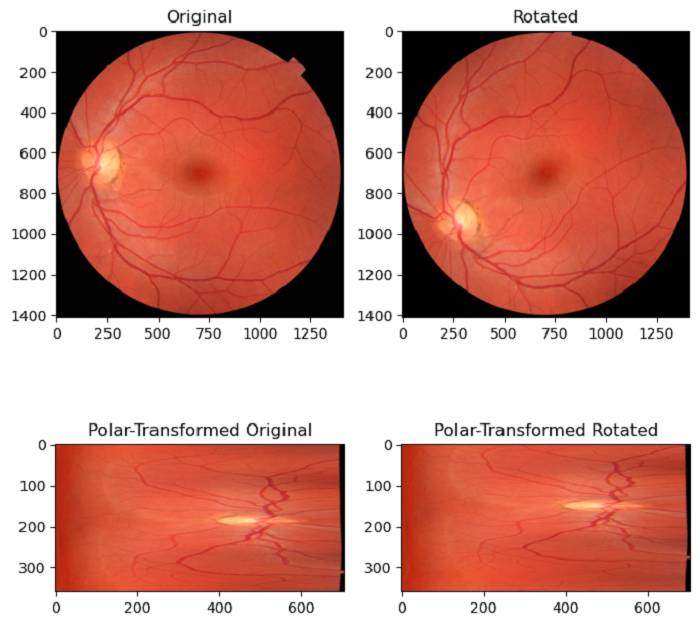
Using the polar transform to recover the rotation difference between two images

In this scenario, we consider the simple case of two images, where the only difference between the images is rotation around a common center point. By transforming these images into polar space, the rotation difference effectively transforms into a straightforward translation difference. This translation difference can be accurately recovered using phase correlation.

Example

Here is an example that demonstrates the use of image registration techniques to recover the rotational difference between two images using the polar transformation.

import numpy as np
import matplotlib.pyplot as plt

from skimage import data
from skimage.registration import phase_cross_correlation
from skimage.transform import warp_polar, rotate, rescale
from skimage.util import img_as_float

polar_radius = 705
rotation_angle = 35

# Load the input image 
original_image = data.retina()

# convert the input image to floating-point format
original_image = img_as_float(original_image)

# rotate the input image 
rotated_image = rotate(original_image, rotation_angle)

# transform the original and rotated images using the warp_polar function
original_polar = warp_polar(original_image, radius=polar_radius, channel_axis=-1)
rotated_polar = warp_polar(rotated_image, radius=polar_radius, channel_axis=-1)

# Display the original and rotated polar images 
fig, axes = plt.subplots(2, 2, figsize=(8, 8))
ax = axes.ravel()

ax[0].set_title("Original")
ax[0].imshow(original_image)

ax[1].set_title("Rotated")
ax[1].imshow(rotated_image)

ax[2].set_title("Polar-Transformed Original")
ax[2].imshow(original_polar)

ax[3].set_title("Polar-Transformed Rotated")
ax[3].imshow(rotated_polar)

plt.show()

# Calculate the translation (shifts) by applying the phase correlation to the original and rotated polar images
shifts, error, phasediff = phase_cross_correlation(original_polar, rotated_polar, normalization=None)
print(f'Expected value for counterclockwise rotation in degrees: '
   f'{rotation_angle}')
print(f'Recovered value for counterclockwise rotation: '
   f'{shifts[0]}')

Output

Expected value for counterclockwise rotation in degrees: 35
Recovered value for counterclockwise rotation: 35.0

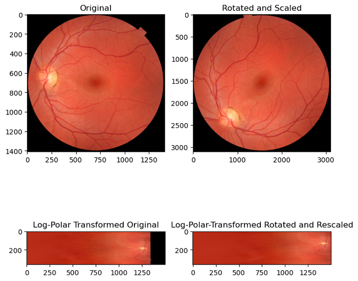
Using the log-polar transform to recover rotation and scaling differences between two images

In this scenario, we consider the images which are differ by both rotation and scaling (note the axis tick values). By transforming these images into log-polar space, we can recover rotation as before, and now also scaling, by phase correlation.

Example

import numpy as np
import matplotlib.pyplot as plt

from skimage import data
from skimage.registration import phase_cross_correlation
from skimage.transform import warp_polar, rotate, rescale
from skimage.util import img_as_float

# Parameters for log-polar transformation, radius must be large enough to capture useful info in larger image
log_polar_radius = 1500
rotation_angle = 53.7
scaling_factor = 2.2

# Load an example image and convert it to a floating-point format
original_image = data.retina()
original_image = img_as_float(original_image)

# Create a rotated and scaled version of the original image
rotated_and_scaled_image = rescale(rotate(original_image, rotation_angle), scaling_factor, channel_axis=-1)

# Perform log-polar transformations on both images
original_log_polar = warp_polar(original_image, radius=log_polar_radius, 
   scaling='log', channel_axis=-1)

rotated_and_scaled_log_polar = warp_polar(rotated_and_scaled_image, radius=log_polar_radius, 
   scaling='log', channel_axis=-1)

# Visualize the images
fig, axes = plt.subplots(2, 2, figsize=(8, 8))
ax = axes.ravel()

ax[0].set_title("Original")
ax[0].imshow(original_image)

ax[1].set_title("Rotated and Scaled")
ax[1].imshow(rotated_and_scaled_image)


ax[2].set_title("Log-Polar Transformed Original")
ax[2].imshow(original_log_polar)

ax[3].set_title("Log-Polar-Transformed Rotated and Rescaled")
ax[3].imshow(rotated_and_scaled_log_polar)

# Apply phase correlation to recover rotation and scaling differences
shifts, error, phasediff = phase_cross_correlation(original_log_polar, rotated_and_scaled_log_polar, 
   upsample_factor=20, normalization=None)

shiftr, shiftc = shifts[:2]

# Calculate scale factor from translation
klog = log_polar_radius / np.log(log_polar_radius)
shift_scale = 1 / (np.exp(shiftc / klog))

print(f'Expected value for cc rotation in degrees: {rotation_angle}')
print(f'Recovered value for cc rotation: {shiftr}')
print()
print(f'Expected value for scaling difference: {scaling_factor}')
print(f'Recovered value for scaling difference: {shift_scale}')

Output

Expected value for cc rotation in degrees: 53.7
Recovered value for cc rotation: 53.75

Expected value for scaling difference: 2.2
Recovered value for scaling difference: 2.1981889915232165