- Scikit Image – Introduction
- Scikit Image - Image Processing
- Scikit Image - Numpy Images
- Scikit Image - Image datatypes
- Scikit Image - Using Plugins
- Scikit Image - Image Handlings
- Scikit Image - Reading Images
- Scikit Image - Writing Images
- Scikit Image - Displaying Images
- Scikit Image - Image Collections
- Scikit Image - Image Stack
- Scikit Image - Multi Image
- Scikit Image - Data Visualization
- Scikit Image - Using Matplotlib
- Scikit Image - Using Ploty
- Scikit Image - Using Mayavi
- Scikit Image - Using Napari
- Scikit Image - Color Manipulation
- Scikit Image - Alpha Channel
- Scikit Image - Conversion b/w Color & Gray Values
- Scikit Image - Conversion b/w RGB & HSV
- Scikit Image - Conversion to CIE-LAB Color Space
- Scikit Image - Conversion from CIE-LAB Color Space
- Scikit Image - Conversion to luv Color Space
- Scikit Image - Conversion from luv Color Space
- Scikit Image - Image Inversion
- Scikit Image - Painting Images with Labels
- Scikit Image - Contrast & Exposure
- Scikit Image - Contrast
- Scikit Image - Contrast enhancement
- Scikit Image - Exposure
- Scikit Image - Histogram Matching
- Scikit Image - Histogram Equalization
- Scikit Image - Local Histogram Equalization
- Scikit Image - Tinting gray-scale images
- Scikit Image - Image Transformation
- Scikit Image - Scaling an image
- Scikit Image - Rotating an Image
- Scikit Image - Warping an Image
- Scikit Image - Affine Transform
- Scikit Image - Piecewise Affine Transform
- Scikit Image - ProjectiveTransform
- Scikit Image - EuclideanTransform
- Scikit Image - Radon Transform
- Scikit Image - Line Hough Transform
- Scikit Image - Probabilistic Hough Transform
- Scikit Image - Circular Hough Transforms
- Scikit Image - Elliptical Hough Transforms
- Scikit Image - Polynomial Transform
- Scikit Image - Image Pyramids
- Scikit Image - Pyramid Gaussian Transform
- Scikit Image - Pyramid Laplacian Transform
- Scikit Image - Swirl Transform
- Scikit Image - Morphological Operations
- Scikit Image - Erosion
- Scikit Image - Dilation
- Scikit Image - Black & White Tophat Morphologies
- Scikit Image - Convex Hull
- Scikit Image - Generating footprints
- Scikit Image - Isotopic Dilation & Erosion
- Scikit Image - Isotopic Closing & Opening of an Image
- Scikit Image - Skelitonizing an Image
- Scikit Image - Morphological Thinning
- Scikit Image - Masking an image
- Scikit Image - Area Closing & Opening of an Image
- Scikit Image - Diameter Closing & Opening of an Image
- Scikit Image - Morphological reconstruction of an Image
- Scikit Image - Finding local Maxima
- Scikit Image - Finding local Minima
- Scikit Image - Removing Small Holes from an Image
- Scikit Image - Removing Small Objects from an Image
- Scikit Image - Filters
- Scikit Image - Image Filters
- Scikit Image - Median Filter
- Scikit Image - Mean Filters
- Scikit Image - Morphological gray-level Filters
- Scikit Image - Gabor Filter
- Scikit Image - Gaussian Filter
- Scikit Image - Butterworth Filter
- Scikit Image - Frangi Filter
- Scikit Image - Hessian Filter
- Scikit Image - Meijering Neuriteness Filter
- Scikit Image - Sato Filter
- Scikit Image - Sobel Filter
- Scikit Image - Farid Filter
- Scikit Image - Scharr Filter
- Scikit Image - Unsharp Mask Filter
- Scikit Image - Roberts Cross Operator
- Scikit Image - Lapalace Operator
- Scikit Image - Window Functions With Images
- Scikit Image - Thresholding
- Scikit Image - Applying Threshold
- Scikit Image - Otsu Thresholding
- Scikit Image - Local thresholding
- Scikit Image - Hysteresis Thresholding
- Scikit Image - Li thresholding
- Scikit Image - Multi-Otsu Thresholding
- Scikit Image - Niblack and Sauvola Thresholding
- Scikit Image - Restoring Images
- Scikit Image - Rolling-ball Algorithm
- Scikit Image - Denoising an Image
- Scikit Image - Wavelet Denoising
- Scikit Image - Non-local means denoising for preserving textures
- Scikit Image - Calibrating Denoisers Using J-Invariance
- Scikit Image - Total Variation Denoising
- Scikit Image - Shift-invariant wavelet denoising
- Scikit Image - Image Deconvolution
- Scikit Image - Richardson-Lucy Deconvolution
- Scikit Image - Recover the original from a wrapped phase image
- Scikit Image - Image Inpainting
- Scikit Image - Registering Images
- Scikit Image - Image Registration
- Scikit Image - Masked Normalized Cross-Correlation
- Scikit Image - Registration using optical flow
- Scikit Image - Assemble images with simple image stitching
- Scikit Image - Registration using Polar and Log-Polar
- Scikit Image - Feature Detection
- Scikit Image - Dense DAISY Feature Description
- Scikit Image - Histogram of Oriented Gradients
- Scikit Image - Template Matching
- Scikit Image - CENSURE Feature Detector
- Scikit Image - BRIEF Binary Descriptor
- Scikit Image - SIFT Feature Detector and Descriptor Extractor
- Scikit Image - GLCM Texture Features
- Scikit Image - Shape Index
- Scikit Image - Sliding Window Histogram
- Scikit Image - Finding Contour
- Scikit Image - Texture Classification Using Local Binary Pattern
- Scikit Image - Texture Classification Using Multi-Block Local Binary Pattern
- Scikit Image - Active Contour Model
- Scikit Image - Canny Edge Detection
- Scikit Image - Marching Cubes
- Scikit Image - Foerstner Corner Detection
- Scikit Image - Harris Corner Detection
- Scikit Image - Extracting FAST Corners
- Scikit Image - Shi-Tomasi Corner Detection
- Scikit Image - Haar Like Feature Detection
- Scikit Image - Haar Feature detection of coordinates
- Scikit Image - Hessian matrix
- Scikit Image - ORB feature Detection
- Scikit Image - Additional Concepts
- Scikit Image - Render text onto an image
- Scikit Image - Face detection using a cascade classifier
- Scikit Image - Face classification using Haar-like feature descriptor
- Scikit Image - Visual image comparison
- Scikit Image - Exploring Region Properties With Pandas
Scikit Image - Histogram Equalization
Histogram is a graphical representation that shows the distribution of pixel intensities of an image. For a digital image histogram plots a graph between pixel intensity versus the number of pixels. The x-axis represents the intensity values, while the y-axis represents the frequency or number of pixels in that particular intensity.
Histogram helps to get a basic idea about image information like contrast, brightness, intensity distribution, etc., by simply looking at the histogram of an image.
Histogram equalization is a technique used to improve the contrast of an image by stretching out the pixel intensities. It can improve the visibility of details and enhance the overall appearance of the image. However, it's important to note that histogram equalization can sometimes yield unnatural-looking images.
In the scikit-image library, the exposure module provides functions for histogram equalization, which are equalize_hist() and equalize_adapthist().
Using the exposure.equalize_hist() function
The exposure.equalize_hist() function is used to perform histogram equalization on an input image. And returns an image after performing the histogram equalization.
Syntax
Following is the syntax of this function −
skimage.exposure.equalize_hist(image, nbins=256, mask=None)
Parameters
- image: The input image array on which histogram equalization will be performed.
- nbins (optional): The number of bins to use for the image histogram. This is ignored for integer images, where each integer is treated as its own bin.
- mask (optional): An array of the same shape as the image, specifying a mask. Only the points where the mask is True will be used for equalization. The equalization is applied to the entire image.
Return Value
It returns an image array after performing the histogram equalization. The array is of type float.
Example
The following example demonstrates how to use the exposure.equalize_hist() function on an image to get the histogram equalization.
import matplotlib.pyplot as plt
from skimage import io, exposure

# Load the input image
image = io.imread('Images/Dog.jpg')

# Perform histogram equalization
equalized_image = exposure.equalize_hist(image)

# Display the original and equalized images
fig, axes = plt.subplots(1, 2, figsize=(10, 5))
axes[0].imshow(image)
axes[0].set_title('Original Image')
axes[0].axis('off')
axes[1].imshow(equalized_image)
axes[1].set_title('Equalized Image')
axes[1].axis('off')

# Show the plot
plt.tight_layout()
plt.show()
Output
On executing the above program, you will get the following output −
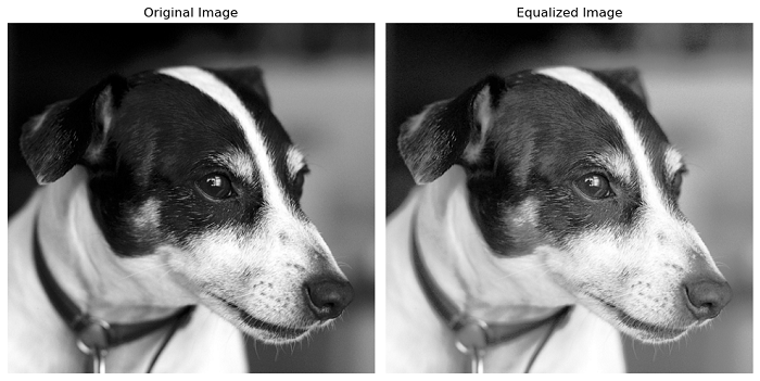
It's important to note that the exposure.equalize_hist() function performs histogram equalization by mapping the cumulative distribution function (CDF) of pixel values onto a linear CDF. This ensures that all parts of the value range are equally represented in the image.
And it leads to enhanced details in large regions with poor contrast. However, to address exposure gradients across the image, a more refined approach can be employed using the equalize_adapthist() function.
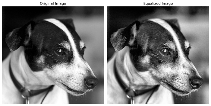
Using the exposure.equalize_adapthist() function
This function implements Contrast Limited Adaptive Histogram Equalization (CLAHE). It is an algorithm for local contrast enhancement that operates on different tile regions of an image's histogram. This allows for the enhancement of local details even in regions that are darker or lighter than the majority of the image.
Syntax
Following is the syntax of this function −
skimage.exposure.equalize_adapthist(image, kernel_size=None, clip_limit=0.01, nbins=256)
Parameters
- image: The input image array (ndarray).
- kernel_size (optional): Defines the shape of contextual regions used in the algorithm. It can be an integer or an array-like object with the same number of elements as the image's dimensions. By default, the kernel size is set to 1/8 of the image's height by 1/8 of its width.
- clip_limit (optional): The clipping limit for contrast normalization, normalized between 0 and 1. Higher values result in more contrast enhancement.
- nbins (optional): The number of gray bins for the histogram.
Return Value
It returns an equalized image with a float64 data type. Note that, the equalize_adapthist() function performs the following steps for color image inputs:
- The image is converted to the HSV color space.
- The CLAHE algorithm is applied to the V (Value) channel.
- The image is converted back to the RGB color space and returned.
- For RGBA images, the original alpha channel is removed.
Example
Here's an example of using the exposure.equalize_adapthist() function on an image.
import matplotlib.pyplot as plt
from skimage import io, exposure

# Load the input image
image = io.imread('Images/Dog.jpg')

# Perform the Adaptive Histogram Equalization
equalized_image = exposure.equalize_adapthist(image)

# Display the original and equalized images
fig, axes = plt.subplots(1, 2, figsize=(10, 5))
axes[0].imshow(image)
axes[0].set_title('Original Image')
axes[0].axis('off')
axes[1].imshow(equalized_image)
axes[1].set_title('Equalized Image')
axes[1].axis('off')

# Show the plot
plt.tight_layout()
plt.show()
Output
On executing the above program, you will get the following output −
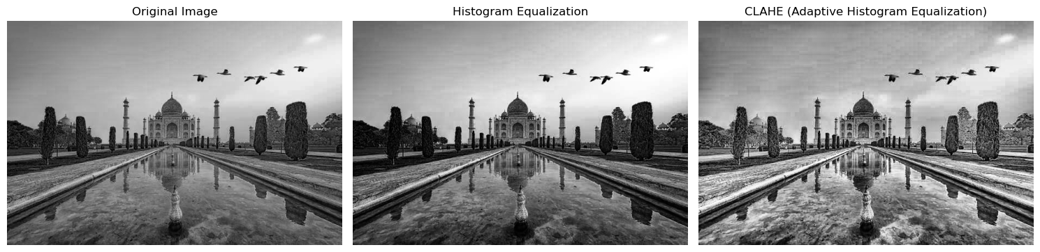
Example
The following example shows, demonstrates the difference between equalize_adapthist() and equalize_hist() methods.
import matplotlib.pyplot as plt
from skimage import io, exposure

# Load the input image
image = io.imread('Images/Blue.jpg', as_gray=True)

# Perform histogram equalization
equalized_hist = exposure.equalize_hist(image)

# Perform CLAHE (Contrast Limited Adaptive Histogram Equalization)
equalized_adapthist = exposure.equalize_adapthist(image)

# Display the original, histogram equalized, and CLAHE equalized images
fig, axes = plt.subplots(1, 3, figsize=(15, 5))
axes[0].imshow(image, cmap='gray')
axes[0].set_title('Original Image')
axes[0].axis('off')
axes[1].imshow(equalized_hist, cmap='gray')
axes[1].set_title('Histogram Equalization')
axes[1].axis('off')
axes[2].imshow(equalized_adapthist, cmap='gray')
axes[2].set_title('CLAHE (Adaptive Histogram Equalization)')
axes[2].axis('off')

# Show the plot
plt.tight_layout()
plt.show()
Output
On executing the above program, you will get the following output −