Scikit Image - Shift-Invariant Wavelet Denoising

Quiz

The concept of shift-invariance is important in signal processing, especially in applications like image denoising, where the denoising algorithm is robust to small shifts or translations in the input signal.

The discrete wavelet transform (DWT) is not inherently shift-invariant. To achieve shift-invariance in wavelet denoising, an undecimated wavelet transform (also called stationary wavelet transform), can be used. However, this approach increases redundancy, resulting in more wavelet coefficients than input image pixels. Another way to approximate shift-invariance in image denoising with the discrete wavelet transform is by using the technique called 'cycle spinning.' This involves averaging the results of the following three steps for multiple spatial shifts, n −

circularly shift the signal by an amount 'n'.
Apply denoising to the shifted signal.
Apply the inverse shift to the denoised signal.

Using the skimage.restoration.cycle_spin() functtion

The scikit-image library provides the dedicated function cycle_spin() within its restoration module for applying cycle spinning. This function repeatedly applies a specified function to shifted versions of x.

Syntax

Following is the syntax of this function −

skimage.restoration.cycle_spin(x, func, max_shifts, shift_steps=1, num_workers=None, func_kw=None, *, channel_axis=None)

Parameters

The function accepts the following parameters −

x (array-like): Input data to which the function func will be applied after circular shifts.
func (function): The function that will be repeatedly applied to circularly shifted versions of x. It should take x as its first argument, and you can provide additional arguments via func_kw.
max_shifts (int or tuple): Specifies the maximum shifts to be applied along each axis of x. It can be an integer or a tuple. If it's an integer, shifts in the range from 0 to max_shifts + 1 will be used along each axis. If it's a tuple, it indicates the maximum shifts along each axis.
shift_steps (int or tuple, optional): The step size for shifts applied along each axis, i, are:: range((0, max_shifts[i]+1, shift_steps[i])). If an integer is provided, the step size is used for all axes.
num_workers (int or None, optional): The number of parallel threads to use during the cycle spinning process. If set to None, it uses the maximum available cores.
func_kw (dict, optional): Additional keyword arguments to be passed to the func function.
channel_axis (int or None, optional): Indicates which axis of the array corresponds to channels. If None, it assumes the image is grayscale (single channel).

The output of the function is (avg_ynp.ndarray) −

The function returns the output of func(x, **func_kw) averaged over all combinations of the specified axis shifts.

Example

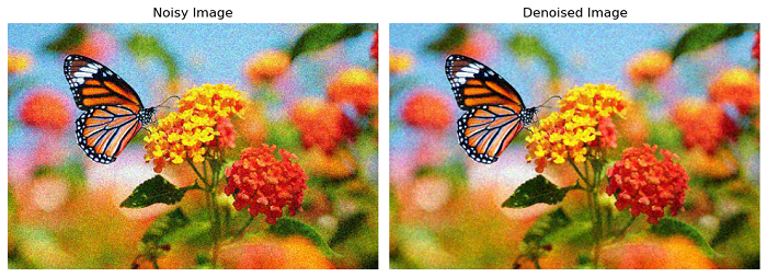
The following example demonstrates a basic image denoising process using shift-invariant wavelet denoising with cycle spinning.

from skimage import io, util
from skimage.restoration import denoise_wavelet, cycle_spin
import numpy as np
import matplotlib.pyplot as plt

# Load the input image from a file
img = util.img_as_float(io.imread('Images/butterfly.jpg'))

# Add Gaussian noise to the image
sigma = 0.1
img_noisy = img + sigma * np.random.standard_normal(img.shape)

# Apply cycle spinning and denoising
denoised = cycle_spin(img_noisy, func=denoise_wavelet, max_shifts=3)

# Visualize the original, noisy, and denoised images
fig, axes = plt.subplots(1, 2, figsize=(10, 5))

# Noisy Image
axes[0].imshow(img_noisy)
axes[0].set_title('Noisy Image')
axes[0].axis('off')

# Denoised Image
axes[1].imshow(denoised)
axes[1].set_title('Denoised Image')
axes[1].axis('off')

plt.tight_layout()
plt.show()

Output

Example

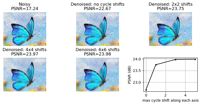
This example demonstrates the process of denoising an image with different degrees of cycle shifting using wavelet denoising and evaluates the Peak Signal-to-Noise Ratio (PSNR) as a measure of denoising quality.

import matplotlib.pyplot as plt
from skimage.restoration import denoise_wavelet, cycle_spin
from skimage import io, util
from skimage.util import random_noise
from skimage.metrics import peak_signal_noise_ratio

# Load the input image and add Gaussian noise
original = util.img_as_float(io.imread('Images/butterfly1.jpg')[22:145, 145:300])
sigma = 0.155
noisy = random_noise(original, var=sigma**2)

# Create a subplot with 2 rows and 3 columns
fig, ax = plt.subplots(nrows=2, ncols=3, figsize=(10, 4),
   sharex=False, sharey=False)
ax = ax.ravel()

# Calculate PSNR for the noisy image and display it
psnr_noisy = peak_signal_noise_ratio(original, noisy)
ax[0].imshow(noisy)
ax[0].axis('off')
ax[0].set_title(f'Noisy&bsol;nPSNR={psnr_noisy:0.4g}')

# Denoise with different amounts of cycle spinning
denoise_kwargs = dict(channel_axis=-1, convert2ycbcr=True, wavelet='db1',
   rescale_sigma=True)
all_psnr = []
max_shifts = [0, 1, 3, 5]
for n, s in enumerate(max_shifts):
   im_bayescs = cycle_spin(noisy, func=denoise_wavelet, max_shifts=s,
      func_kw=denoise_kwargs, channel_axis=-1)
   ax[n+1].imshow(im_bayescs)
   ax[n+1].axis('off')
   psnr = peak_signal_noise_ratio(original, im_bayescs)
   if s == 0:
      ax[n+1].set_title(
         f'Denoised: no cycle shifts&bsol;nPSNR={psnr:0.4g}')
   else:
      ax[n+1].set_title(
         f'Denoised: {s+1}x{s+1} shifts&bsol;nPSNR={psnr:0.4g}')
   all_psnr.append(psnr)

# Plot PSNR as a function of the degree of cycle shifting
ax[5].plot(max_shifts, all_psnr, 'k.-')
ax[5].set_ylabel('PSNR (dB)')
ax[5].set_xlabel('max cycle shift along each axis')
ax[5].grid(True)

# Adjust subplot spacing
plt.subplots_adjust(wspace=0.35, hspace=0.35)

plt.show()

Output

Print Page