- Scikit Image – Introduction
- Scikit Image - Image Processing
- Scikit Image - Numpy Images
- Scikit Image - Image datatypes
- Scikit Image - Using Plugins
- Scikit Image - Image Handlings
- Scikit Image - Reading Images
- Scikit Image - Writing Images
- Scikit Image - Displaying Images
- Scikit Image - Image Collections
- Scikit Image - Image Stack
- Scikit Image - Multi Image
- Scikit Image - Data Visualization
- Scikit Image - Using Matplotlib
- Scikit Image - Using Ploty
- Scikit Image - Using Mayavi
- Scikit Image - Using Napari
- Scikit Image - Color Manipulation
- Scikit Image - Alpha Channel
- Scikit Image - Conversion b/w Color & Gray Values
- Scikit Image - Conversion b/w RGB & HSV
- Scikit Image - Conversion to CIE-LAB Color Space
- Scikit Image - Conversion from CIE-LAB Color Space
- Scikit Image - Conversion to luv Color Space
- Scikit Image - Conversion from luv Color Space
- Scikit Image - Image Inversion
- Scikit Image - Painting Images with Labels
- Scikit Image - Contrast & Exposure
- Scikit Image - Contrast
- Scikit Image - Contrast enhancement
- Scikit Image - Exposure
- Scikit Image - Histogram Matching
- Scikit Image - Histogram Equalization
- Scikit Image - Local Histogram Equalization
- Scikit Image - Tinting gray-scale images
- Scikit Image - Image Transformation
- Scikit Image - Scaling an image
- Scikit Image - Rotating an Image
- Scikit Image - Warping an Image
- Scikit Image - Affine Transform
- Scikit Image - Piecewise Affine Transform
- Scikit Image - ProjectiveTransform
- Scikit Image - EuclideanTransform
- Scikit Image - Radon Transform
- Scikit Image - Line Hough Transform
- Scikit Image - Probabilistic Hough Transform
- Scikit Image - Circular Hough Transforms
- Scikit Image - Elliptical Hough Transforms
- Scikit Image - Polynomial Transform
- Scikit Image - Image Pyramids
- Scikit Image - Pyramid Gaussian Transform
- Scikit Image - Pyramid Laplacian Transform
- Scikit Image - Swirl Transform
- Scikit Image - Morphological Operations
- Scikit Image - Erosion
- Scikit Image - Dilation
- Scikit Image - Black & White Tophat Morphologies
- Scikit Image - Convex Hull
- Scikit Image - Generating footprints
- Scikit Image - Isotopic Dilation & Erosion
- Scikit Image - Isotopic Closing & Opening of an Image
- Scikit Image - Skelitonizing an Image
- Scikit Image - Morphological Thinning
- Scikit Image - Masking an image
- Scikit Image - Area Closing & Opening of an Image
- Scikit Image - Diameter Closing & Opening of an Image
- Scikit Image - Morphological reconstruction of an Image
- Scikit Image - Finding local Maxima
- Scikit Image - Finding local Minima
- Scikit Image - Removing Small Holes from an Image
- Scikit Image - Removing Small Objects from an Image
- Scikit Image - Filters
- Scikit Image - Image Filters
- Scikit Image - Median Filter
- Scikit Image - Mean Filters
- Scikit Image - Morphological gray-level Filters
- Scikit Image - Gabor Filter
- Scikit Image - Gaussian Filter
- Scikit Image - Butterworth Filter
- Scikit Image - Frangi Filter
- Scikit Image - Hessian Filter
- Scikit Image - Meijering Neuriteness Filter
- Scikit Image - Sato Filter
- Scikit Image - Sobel Filter
- Scikit Image - Farid Filter
- Scikit Image - Scharr Filter
- Scikit Image - Unsharp Mask Filter
- Scikit Image - Roberts Cross Operator
- Scikit Image - Lapalace Operator
- Scikit Image - Window Functions With Images
- Scikit Image - Thresholding
- Scikit Image - Applying Threshold
- Scikit Image - Otsu Thresholding
- Scikit Image - Local thresholding
- Scikit Image - Hysteresis Thresholding
- Scikit Image - Li thresholding
- Scikit Image - Multi-Otsu Thresholding
- Scikit Image - Niblack and Sauvola Thresholding
- Scikit Image - Restoring Images
- Scikit Image - Rolling-ball Algorithm
- Scikit Image - Denoising an Image
- Scikit Image - Wavelet Denoising
- Scikit Image - Non-local means denoising for preserving textures
- Scikit Image - Calibrating Denoisers Using J-Invariance
- Scikit Image - Total Variation Denoising
- Scikit Image - Shift-invariant wavelet denoising
- Scikit Image - Image Deconvolution
- Scikit Image - Richardson-Lucy Deconvolution
- Scikit Image - Recover the original from a wrapped phase image
- Scikit Image - Image Inpainting
- Scikit Image - Registering Images
- Scikit Image - Image Registration
- Scikit Image - Masked Normalized Cross-Correlation
- Scikit Image - Registration using optical flow
- Scikit Image - Assemble images with simple image stitching
- Scikit Image - Registration using Polar and Log-Polar
- Scikit Image - Feature Detection
- Scikit Image - Dense DAISY Feature Description
- Scikit Image - Histogram of Oriented Gradients
- Scikit Image - Template Matching
- Scikit Image - CENSURE Feature Detector
- Scikit Image - BRIEF Binary Descriptor
- Scikit Image - SIFT Feature Detector and Descriptor Extractor
- Scikit Image - GLCM Texture Features
- Scikit Image - Shape Index
- Scikit Image - Sliding Window Histogram
- Scikit Image - Finding Contour
- Scikit Image - Texture Classification Using Local Binary Pattern
- Scikit Image - Texture Classification Using Multi-Block Local Binary Pattern
- Scikit Image - Active Contour Model
- Scikit Image - Canny Edge Detection
- Scikit Image - Marching Cubes
- Scikit Image - Foerstner Corner Detection
- Scikit Image - Harris Corner Detection
- Scikit Image - Extracting FAST Corners
- Scikit Image - Shi-Tomasi Corner Detection
- Scikit Image - Haar Like Feature Detection
- Scikit Image - Haar Feature detection of coordinates
- Scikit Image - Hessian matrix
- Scikit Image - ORB feature Detection
- Scikit Image - Additional Concepts
- Scikit Image - Render text onto an image
- Scikit Image - Face detection using a cascade classifier
- Scikit Image - Face classification using Haar-like feature descriptor
- Scikit Image - Visual image comparison
- Scikit Image - Exploring Region Properties With Pandas
Scikit Image - Dilation
Dilation is a fundamental operation in mathematical morphology that increases the size of bright regions and shrinks dark regions in an image. This is done by setting the value of a pixel to the maximum value over all the pixels in its neighborhood defined by a structuring element. And it is widely used in image processing tasks, including expanding object boundaries, filling small gaps, noise reduction, object enlargement, and feature enhancement.
The scikit-image library provides the functions like morphology.dilation() and morphology.binary_dilation() to perform dilation and binary dilation operations on images.
Using the skimage.morphology.dilation() function
The morphology.dilation() function is used for grayscale morphological dilation of an image. It works by setting the pixel values in the output image to the maximum overall pixel values within a local neighborhood centered around it.
Syntax
Following is the syntax of this function −
skimage.morphology.dilation(image, footprint=None, out=None, shift_x=False, shift_y=False)
Parameters
- image (ndarray): This is the input image on which dilation will be performed.
- footprint (ndarray or tuple, optional): The neighborhood to be used for dilation, expressed as a 2-D array of 1s and 0s. If None is provided, a cross-shaped footprint (connectivity=1) is used. You can also specify a custom footprint as a sequence of smaller footprints. For example, footprint=[(np.ones((9, 1)), 1), (np.ones((1, 9)), 1)] would apply a 9x1 footprint followed by a 1x9 footprint, resulting in a net effect that is the same as footprint=np.ones((9, 9)). This can help reduce the computational cost for certain footprints.
- out (ndarray, optional): The output array where the result of the morphology will be stored. If None is passed, a new array will be allocated for the result.
- shift_x and shift_y (bool, optional): These parameters control whether the footprint should be shifted about the center point. This only affects eccentric footprints (i.e., footprints with even-numbered sides).
Return Value
It returns a dilated array of the same shape and type as the input image.
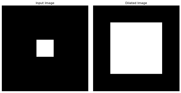
Example
The following example demonstrates how to use the dilation() function on an image.
import numpy as np
import matplotlib.pyplot as plt
from skimage.morphology import square, dilation

# Create an example input image
bright_pixel = np.array([[0, 0, 0, 0, 0],
                         [0, 0, 0, 0, 0],
                         [0, 0, 1, 0, 0],
                         [0, 0, 0, 0, 0],
                         [0, 0, 0, 0, 0]], dtype=np.uint8)

# Perform dilation using a square-shaped footprint of size 3x3
result = dilation(bright_pixel, square(3))

# Create subplots to display the input and dilated images
fig, axes = plt.subplots(1, 2, figsize=(10, 5))
ax = axes.ravel()

# Display the input image
ax[0].imshow(bright_pixel, cmap=plt.cm.gray)
ax[0].set_title('Input Image')
ax[0].set_axis_off()

# Display the eroded image
ax[1].imshow(result, cmap=plt.cm.gray)
ax[1].set_title('Dilated Image')
ax[1].set_axis_off()

plt.tight_layout()
plt.show()
Output
On executing the above program, you will get the following output −
Using the skimage.morphology.binary_dilation() function
The morphology.binary_dilation() function is used for fast binary morphological dilation of a binary image. Binary dilation is similar to grayscale dilation, but it works faster for binary images. It enlarges the bright regions and shrinks the dark regions.
Syntax
Following is the syntax of this function −
skimage.morphology.binary_dilation(image, footprint=None, out=None)
Parameters
- image (ndarray): This is the binary input image on which dilation will be performed.
- footprint (ndarray or tuple, optional): The neighborhood to be used for dilation, expressed as a 2-D array of 1s and 0s. If None is provided, a cross-shaped footprint (connectivity=1) is used. You can also specify a custom footprint as a sequence of smaller footprints, which can help reduce computational cost for certain footprints.
- out (ndarray, optional): The output array where the result of the morphology will be stored. If None is passed, a new array will be allocated for the result.
Return Value
It returns a dilated binary image with values in [False, True].
Example
Here is an example that demonstrates how to use the binary_dilation() function on an image.
import numpy as np
import matplotlib.pyplot as plt
from skimage.morphology import square, binary_dilation

# Create an example binary input image
binary_pixel = np.array([[0, 0, 0, 0, 0],
                         [0, 0, 0, 0, 0],
                         [0, 0, 1, 0, 0],
                         [0, 0, 0, 0, 0],
                         [0, 0, 0, 0, 0]], dtype=np.uint8)

# Perform binary dilation using a square-shaped footprint of size 3x3
result = binary_dilation(binary_pixel, square(3))

# Create subplots to display the input and dilated binary images
fig, axes = plt.subplots(1, 2, figsize=(10, 5))
ax = axes.ravel()

# Display the input image
ax[0].imshow(binary_pixel, cmap=plt.cm.gray)
ax[0].set_title('Input Image')
ax[0].set_axis_off()

# Display the eroded image
ax[1].imshow(result, cmap=plt.cm.gray)
ax[1].set_title('Dilated Binary Image')
ax[1].set_axis_off()

plt.tight_layout()
plt.show()
Output
On executing the above program, you will get the following output −

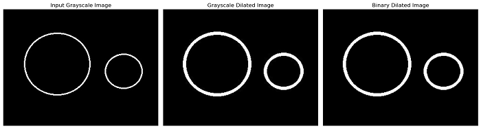
Example
The following example performs both the grayscale and binary dilation on an image using the morphology.dilation() and morphology.binary_dilation() functions respectively.
import numpy as np
import matplotlib.pyplot as plt
from skimage.morphology import disk, dilation, binary_dilation
from skimage import io, color
from skimage.util import img_as_ubyte

# Load a grayscale input image
image = io.imread('Images/Circle2.jpg', as_gray=True)

# Create a binary image
threshold_value = 0.5
binary_image = image > threshold_value

# Perform grayscale dilation using a disk-shaped structuring element of radius 5
grayscale_dilated = dilation(image, disk(2))

# Perform binary dilation using a disk-shaped structuring element of radius 2
binary_dilated = binary_dilation(binary_image, disk(2))

# Create subplots to display the input, grayscale dilated, and binary dilated images
fig, axes = plt.subplots(1, 3, figsize=(15, 5))
ax = axes.ravel()

# Display the input grayscale image
ax[0].imshow(image, cmap=plt.cm.gray)
ax[0].set_title('Input Grayscale Image')
ax[0].set_axis_off()

# Display the grayscale dilated image
ax[1].imshow(grayscale_dilated, cmap=plt.cm.gray)
ax[1].set_title('Grayscale Dilated Image')
ax[1].set_axis_off()

# Display the binary dilated image
ax[2].imshow(binary_dilated, cmap=plt.cm.gray)
ax[2].set_title('Binary Dilated Image')
ax[2].set_axis_off()

plt.tight_layout()
plt.show()
Output
On executing the above program, you will get the following output −