Scikit Image - BRIEF Binary Descriptor

Quiz

BRIEF (Binary Robust Independent Elementary Features) is an efficient feature(keypoint) point descriptor commonly used in computer vision and image processing tasks. This descriptor is known for its high discriminative power, even with a relatively small number of bits. It computes descriptors using straightforward intensity difference tests.

For each keypoint, BRIEF performs intensity comparisons on a specifically distributed number, N, of pixel pairs. This process generates a binary descriptor of length N. When working with binary descriptors, feature matching is typically done using the Hamming distance metric, which offers advantages in terms of computational efficiency compared to the L2 norm.

This short binary descriptor, results in a low memory footprint and efficient matching based on the Hamming distance metric. It's important to note that BRIEF does not inherently offer rotation-invariance, but scale-invariance can be achieved by detecting and extracting features at different scales.

Using the skimage.feature.BRIEF() class

The Scikit-image library provides a flexible way to use the BRIEF binary descriptor through the skimage.feature.BRIEF() class.

Syntax

Following is the syntax of this class −

class skimage.feature.BRIEF(descriptor_size=256, patch_size=49, mode='normal', sigma=1, rng=1)

Parameters

Here are the parameters of the class −

descriptor_size (int, optional): Size of the BRIEF descriptor for each keypoint. The authors recommend using sizes like 128, 256, or 512. The default size is 256.
patch_size (int, optional): The length of the two-dimensional square patch sampling region around keypoints. The default is 49.
mode (str, optional): Probability distribution for sampling the location of decision pixel-pairs around keypoints. It can take one of two values: 'normal' or 'uniform'. The default mode is 'normal'.
rng (numpy.random.Generator or int, optional): Pseudo-random number generator (RNG) used for random sampling of decision pixel-pairs. By default, it uses a PCG64 generator. If y rng is an integer value, it is used to seed the generator. It's important to use the same RNG when constructing descriptors for matching across images.
sigma (float, optional): Standard deviation of the Gaussian low-pass filter applied to the image to reduce sensitivity to noise. Using a low-pass filter is strongly recommended for obtaining discriminative and robust descriptors. The default value is 1.

The class has the following attributes and methods −

Attributes

descriptors ((Q, descriptor_size) array of dtype bool): This attribute stores the binary descriptors. It's a 2D ndarray of binary descriptors of size descriptor_size for Q keypoints after filtering out border keypoints. The value at an index (i, j) is either True or False, representing the outcome of the intensity comparison for the i-th keypoint on the j-th decision pixel-pair. And Q should be equal to np.sum(mask).
mask ((N,) array of dtype bool): This attribute is a mask indicating whether a keypoint has been filtered out (False) or is described in the descriptors array (True). The length of the mask N corresponds to the number of keypoints.

Method

extract(image, keypoints): It extracts BRIEF binary descriptors for given keypoints in an input image.

image (2D array): The input image on which BRIEF descriptors are extracted.
keypoints ((N, 2) array): This parameter represents the keypoints coordinates as (row, col) pairs.

Example

Here is a simple example that performs the keypoint detection, descriptor extraction, and matching using the BRIEF binary description algorithm.

from skimage.feature import (corner_harris, corner_peaks, BRIEF, match_descriptors)
import numpy as np

# Create two squares with different sizes
square1 = np.zeros((8, 8), dtype=np.int32)
square1[2:6, 2:6] = 1
square2 = np.zeros((9, 9), dtype=np.int32)
square2[2:7, 2:7] = 1

print("square1:")
print(square1)
print("square2:")
print(square2)

# Detect Harris corners in both squares
keypoints1 = corner_peaks(corner_harris(square1), min_distance=1)
keypoints2 = corner_peaks(corner_harris(square2), min_distance=1)

# Initialize the BRIEF descriptor extractor with a patch size of 5
extractor = BRIEF(patch_size=5)

# Extract descriptors for keypoints in square1
extractor.extract(square1, keypoints1)
descriptors1 = extractor.descriptors

# Extract descriptors for keypoints in square2
extractor.extract(square2, keypoints2)
descriptors2 = extractor.descriptors

# Match the descriptors between square1 and square2
matches = match_descriptors(descriptors1, descriptors2)

# Print the matches
print("Matches:")
print(matches)

# Get the corresponding keypoints for the matched descriptors
matched_keypoints1 = keypoints1[matches[:, 0]]
matched_keypoints2 = keypoints2[matches[:, 1]]

# Print the matched keypoints
print("Matched Keypoints in square1:")
print(matched_keypoints1)
print("Matched Keypoints in square2:")
print(matched_keypoints2)

Output

On executing the above program, you will get the following output −

square1:
[[0 0 0 0 0 0 0 0]
 [0 0 0 0 0 0 0 0]
 [0 0 1 1 1 1 0 0]
 [0 0 1 1 1 1 0 0]
 [0 0 1 1 1 1 0 0]
 [0 0 1 1 1 1 0 0]
 [0 0 0 0 0 0 0 0]
 [0 0 0 0 0 0 0 0]]

square2:
[[0 0 0 0 0 0 0 0 0]
 [0 0 0 0 0 0 0 0 0]
 [0 0 1 1 1 1 1 0 0]
 [0 0 1 1 1 1 1 0 0]
 [0 0 1 1 1 1 1 0 0]
 [0 0 1 1 1 1 1 0 0]
 [0 0 1 1 1 1 1 0 0]
 [0 0 0 0 0 0 0 0 0]
 [0 0 0 0 0 0 0 0 0]]

Matches:
[[0 0]
 [1 1]
 [2 2]
 [3 3]]

Matched Keypoints in square1:
[[2 2]
 [2 5]
 [5 2]
 [5 5]]

Matched Keypoints in square2:
[[2 2]
 [2 6]
 [6 2]
 [6 6]]

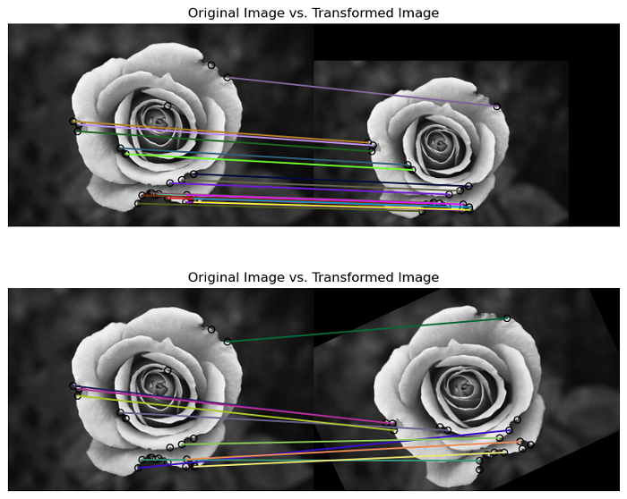
Example

This example demonstrates the BRIEF binary description algorithm using the skimage.feature.BRIEF() class.

import numpy as np
import matplotlib.pyplot as plt
from skimage import transform
from skimage.feature import (match_descriptors, corner_peaks, corner_harris, plot_matches, BRIEF)
from skimage import io, color

# load the input image and convert it to grayscale
img1= color.rgb2gray(io.imread('Images/black rose.jpg'))

# Apply transformations to create img2 and img3
tform = transform.AffineTransform(scale=(1.2, 1.2), translation=(0, -100))
img2 = transform.warp(img1, tform)
img3 = transform.rotate(img1, 25)

# Perform corner detection on all images
keypoints1 = corner_peaks(corner_harris(img1), min_distance=5, threshold_rel=0.1)
keypoints2 = corner_peaks(corner_harris(img2), min_distance=5, threshold_rel=0.1)
keypoints3 = corner_peaks(corner_harris(img3), min_distance=5, threshold_rel=0.1)

# Initialize the BRIEF descriptor extractor
extractor = BRIEF()

# Extract descriptors for all images and keypoints
extractor.extract(img1, keypoints1)
keypoints1 = keypoints1[extractor.mask]
descriptors1 = extractor.descriptors

extractor.extract(img2, keypoints2)
keypoints2 = keypoints2[extractor.mask]
descriptors2 = extractor.descriptors

extractor.extract(img3, keypoints3)
keypoints3 = keypoints3[extractor.mask]
descriptors3 = extractor.descriptors

# Perform descriptor matching for img1 vs. img2 and img1 vs. img3
matches12 = match_descriptors(descriptors1, descriptors2, cross_check=True)
matches13 = match_descriptors(descriptors1, descriptors3, cross_check=True)

# Display the matching results
fig, ax = plt.subplots(nrows=2, ncols=1, figsize=(10,8))
plt.gray()

plot_matches(ax[0], img1, img2, keypoints1, keypoints2, matches12)
ax[0].axis('off')
ax[0].set_title("Original Image vs. Transformed Image")

plot_matches(ax[1], img1, img3, keypoints1, keypoints3, matches13)
ax[1].axis('off')
ax[1].set_title("Original Image vs. Transformed Image")
plt.show()

Output

Print Page