Scikit Image - Visual Image Comparison

Quiz

Visual image comparison, in general, involves the process of visually inspecting and evaluating two or more images with the human eye. This process requires placing the images side by side or overlaying them to observe and analyze the differences and similarities between them.

Visual image comparison is a valuable technique in the field of image processing, especially when dealing with tasks such as adjusting exposure, applying filters, and restoring images.

The scikit-image library offers the compare_images() function within its util module to perform the Visual image comparison tasks on images.

Using the skimage.util.compare_images() function

This function is used to compare two images and generate a new image that shows the differences between them.

Syntax

Here is the syntax of the function −

skimage.util.compare_images(image1, image2, method='diff', *, n_tiles=(8, 8))

Parameters

Following are the parameters of the function −

image1 and image2 (2-D arrays): These are the two input images that you want to compare. They must be of the same shape.
method (string, optional): This parameter specifies the method used for the image comparison. It accepts one of the following values −
- 'diff': This method computes the absolute difference between the two input images.
- 'blend': This method computes the mean (average) value of pixel intensities between the two input images.
- 'checkerboard': This method creates a checkerboard pattern by dividing the image into tiles, where each tile alternates between displaying parts of the first and second input images.
- n_tiles (tuple, optional): This parameter is only used when the method is set to 'checkerboard'. It specifies the number of tiles in the checkerboard pattern, with the format (rows, columns).

The function returns a 2-D array, which is an image showing the differences between the two input images based on the selected comparison method.

let's see the various approaches for comparing two images −

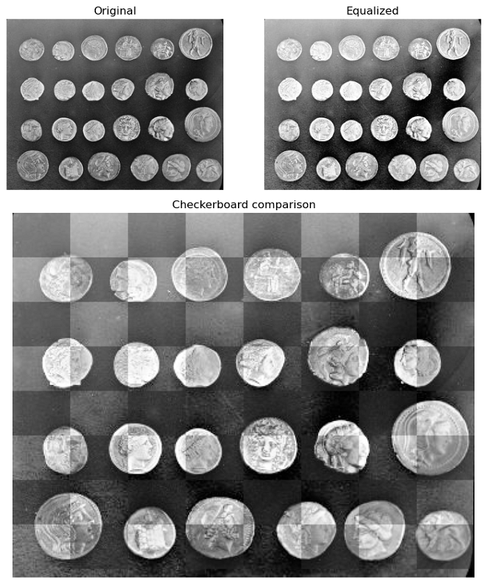
Checkerboard

The checkerboard method involves creating a pattern of alternating tiles or squares that display portions of the first and the second images being compared.

Example

The following example demonstrates how to perform image comparison using a checkerboard pattern.

import matplotlib.pyplot as plt
from matplotlib.gridspec import GridSpec
from skimage import data, transform, exposure
from skimage.util import compare_images

# Load the original image and perform histogram equalization
original_image = data.coins()
equalized_image = exposure.equalize_hist(original_image)

# Rotate the original image
rotated_image = transform.rotate(original_image, 2)

# Compare the original and equalized images using the checkerboard method
comparison_image = compare_images(original_image, equalized_image, method='checkerboard')

# Create a visual comparison display
fig = plt.figure(figsize=(8, 9))
grid_spec = GridSpec(3, 2)

# Subplots for original and equalized images
ax0 = fig.add_subplot(grid_spec[0, 0])
ax1 = fig.add_subplot(grid_spec[0, 1])

# Subplot for the checkerboard comparison
ax2 = fig.add_subplot(grid_spec[1:, :])

# Display the original image
ax0.imshow(original_image, cmap='gray')
ax0.set_title('Original')

# Display the equalized image
ax1.imshow(equalized_image, cmap='gray')
ax1.set_title('Equalized')

# Display the checkerboard comparison
ax2.imshow(comparison_image, cmap='gray')
ax2.set_title('Checkerboard comparison')

# Turn off axes for all subplots
for a in (ax0, ax1, ax2):
   a.axis('off')

plt.tight_layout()
plt.show()

Output

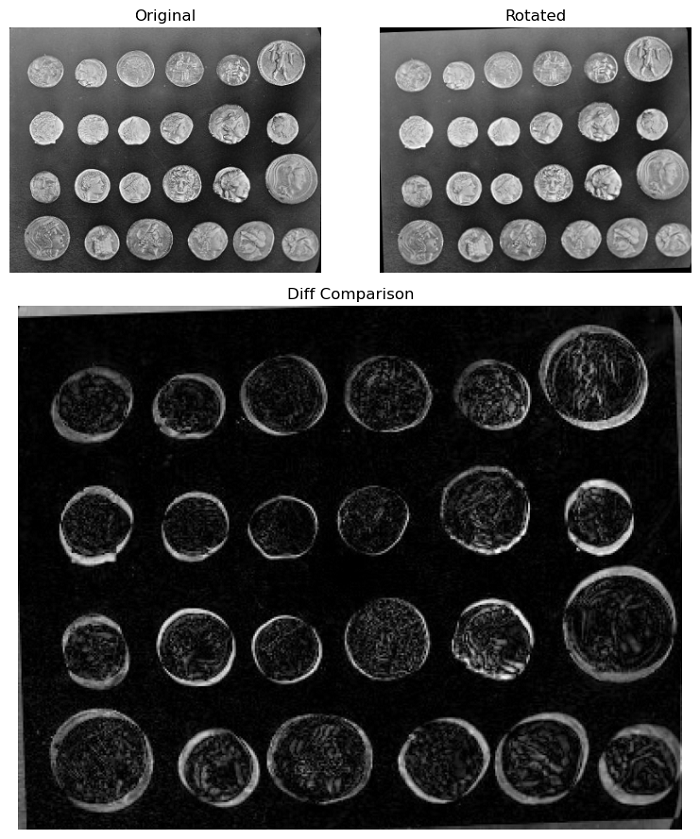
Diff

The diff method computes the absolute difference between the two images to determine how much they vary from each other.

Example

Here is an example that applies the diff method to compare the two images.

import matplotlib.pyplot as plt
from matplotlib.gridspec import GridSpec
from skimage import data, transform, exposure
from skimage.util import compare_images

# Load the coins image and perform histogram equalization
original_image = data.coins()
equalized_image = exposure.equalize_hist(original_image)

# Rotate the original image
rotated_image = transform.rotate(original_image, 2)

# Compare the original and rotated images using the "diff" method
comparison_image = compare_images(original_image, rotated_image, method='diff')

# Create a visual comparison display
fig = plt.figure(figsize=(8, 9))
grid_spec = GridSpec(3, 2)

# Subplots for original and rotated images
ax0 = fig.add_subplot(grid_spec[0, 0])
ax1 = fig.add_subplot(grid_spec[0, 1])

# Subplot for the "diff" comparison
ax2 = fig.add_subplot(grid_spec[1:, :])

# Display the original image
ax0.imshow(original_image, cmap='gray')
ax0.set_title('Original')

# Display the rotated image
ax1.imshow(rotated_image, cmap='gray')
ax1.set_title('Rotated')

# Display the "diff" comparison
ax2.imshow(comparison_image, cmap='gray')
ax2.set_title('Diff Comparison')

for a in (ax0, ax1, ax2):
   a.axis('off')

plt.tight_layout()
plt.show()

Output

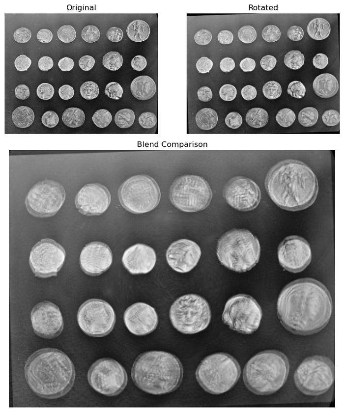
Blend

The blend method in image comparison calculates the average of pixel values from two images.

Example

Here is an example the demonstrates how to use the compare_images() function to perform a visual image comparison with the "blend" method.

import matplotlib.pyplot as plt
from matplotlib.gridspec import GridSpec
from skimage import data, transform, exposure
from skimage.util import compare_images

# Load the coins image and perform histogram equalization
original_image = data.coins()
equalized_image = exposure.equalize_hist(original_image)

# Rotate the original image
rotated_image = transform.rotate(original_image, 2)

# Compare the original and rotated images using the blend method
comparison_image = compare_images(original_image, rotated_image, method='blend')

# Create a visual comparison display
fig = plt.figure(figsize=(8, 9))
grid_spec = GridSpec(3, 2)

# Subplots for original and equalized images
ax0 = fig.add_subplot(grid_spec[0, 0])
ax1 = fig.add_subplot(grid_spec[0, 1])

# Subplot for the Blend comparison
ax2 = fig.add_subplot(grid_spec[1:, :])

ax0.imshow(original_image, cmap='gray')
ax0.set_title('Original')
ax1.imshow(rotated_image, cmap='gray')
ax1.set_title('Rotated')
ax2.imshow(comparison_image, cmap='gray')
ax2.set_title('Blend Comparison')

# Turn off axes for all subplots
for a in (ax0, ax1, ax2):
   a.axis('off')

plt.tight_layout()
plt.show()

Output

Print Page