Scikit Image - Line Hough Transform

Quiz

The Hough Transform is a technique used in image analysis and computer vision to detect shapes, patterns, or structures within an image that can be represented in a mathematical form. And the Line Hough Transform is a specific version of this technique that focuses on identifying lines.

In the context of lines, the Hough Transform works by transforming the lines ( y = mx + b) into a parameter space representation (Hough space) where lines are represented by points. Each point in Hough space corresponds to a possible line in the original image.

In the scikit-image library, the Line Hough Transform can be performed using the transform.hough_line() function, it applies the Line Hough Transform and returns the hough space accumulator, as well as the angles and distances corresponding to the detected lines.

Once you have the accumulator array, you can use the transform.hough_line_peaks() function to find the strongest signals (peaks) in the accumulator. These peaks represent the detected lines, and the angles and distances can be used to reconstruct the lines in the original image space.

Using the skimage.transform.hough_line() function

This function is used to perform a straight line Hough transform on an input image.

Syntax

Following is the syntax of this function −

skimage.transform.hough_line(image, theta=None)

Parameters

image: This parameter should be a 2D NumPy array (ndarray) representing the input image with nonzero values indicating edges. This means that the image should be a binary image where edges are marked with non-zero values and the rest is zero.
theta (optional): An optional parameter that specifies the angles at which to compute the Hough transform. It is a 1D NumPy array of double values representing angles in radians. By default, it generates a vector of 180 angles evenly spaced in the range from -pi/2 to pi/2.
circle (optional): A boolean flag that determines whether to assume the image is zero outside the inscribed circle. If set to True, the width of each projection in the resulting sinogram will be equal to the minimum of the image's width and height.

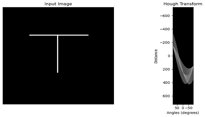
Example

Here is an example that demonstrates how to apply the Hough transform to an input image using the hough_line() function.

import numpy as np
import matplotlib.pyplot as plt
from skimage import transform, io

# Load an input image
image = io.imread('Images/text_image.png', as_gray=True)

# Apply the Hough transform
hspace, angles, distances = transform.hough_line(image)

# Plot the original and transformed images side by side
fig, axes = plt.subplots(1, 2, figsize=(10, 5))
axes[0].imshow(image, cmap='gray')
axes[0].set_title('Input Image')
axes[0].axis('off')

axes[1].imshow(np.log(1 + hspace),
           extent=[np.rad2deg(angles[-1]), np.rad2deg(angles[0]), distances[-1], distances[0]],
           cmap=plt.cm.gray, aspect=1/1.5)
axes[1].set_title('Hough Transform')
axes[1].set_xlabel('Angles (degrees)')
axes[1].set_ylabel('Distance')
plt.tight_layout()
plt.show()

Output

On executing the above program, you will get the following output −

Using the skimage.transform.hough_line_peaks() function

This function is used to identify prominent peaks in the Hough space obtained from the straight line Hough transform. This function helps you find the most significant lines separated by a certain angle and distance in a Hough transform.

Syntax

Following is the syntax of this function −

skimage.transform.hough_line_peaks(hspace, angles, dists, min_distance=9, min_angle=10, threshold=None, num_peaks=inf)

Parameters

hspace: A 2D array representing the Hough space generated by the hough_line() function.
angles: An array of angles returned by the hough_line function. These angles correspond to the detected lines in radians.
dists: An array of distances returned by the hough_line function. These distances represent the distances from the origin to the detected lines.
min_distance: An optional parameter that specifies the minimum distance separating lines. It determines the maximum filter size for the first dimension of the Hough space.
min_angle: An optional parameter that specifies the minimum angle separating lines. It determines the maximum filter size for the second dimension of the Hough space.
threshold: An optional parameter that defines the minimum intensity of peaks to be considered. The default threshold is set to 0.5 times the maximum value in the Hough space.
num_peaks: An optional parameter that specifies the maximum number of peaks to be returned. When the number of detected peaks exceeds this value, only the num_peaks coordinates with the highest peak intensities are returned.

Return Value

It returns a tuple of arrays containing the peak values in the Hough space, the corresponding angles, and the distances. These peaks represent the most prominent lines identified by the Hough transform.

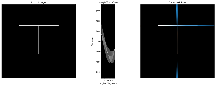
Example

In this following example we will see how to detect peaks in the Hough space using the hough_line_peaks() function.

import numpy as np
import matplotlib.pyplot as plt
from skimage import transform, io

# Load an input image
image = io.imread('Images/text_image.png', as_gray=True)

# Set a precision of 0.05 degree.
tested_angles = np.linspace(-np.pi / 2, np.pi / 2, 360, endpoint=False)

# Apply Classic straight-line Hough transform
hspace, angles, distances = transform.hough_line(image, theta=tested_angles)

# Plot the original and transformed images side by side
fig, axes = plt.subplots(1, 3, figsize=(15, 6))
axes[0].imshow(image, cmap='gray')
axes[0].set_title('Input Image')
axes[0].axis('off')

axes[1].imshow(np.log(1 + hspace),
           extent=[np.rad2deg(angles[-1]), np.rad2deg(angles[0]), distances[-1], distances[0]],
           cmap=plt.cm.gray, aspect=1/1.5)
axes[1].set_title('Hough Transform')
axes[1].set_xlabel('Angles (degrees)')
axes[1].set_ylabel('Distance')

axes[2].imshow(image, cmap='gray')
axes[2].set_ylim((image.shape[0], 0))
axes[2].set_axis_off()
axes[2].set_title('Detected lines')

# Find peaks in the Hough space using the hough_line_peaks() function
for accum, angle, dist in zip(*transform.hough_line_peaks(hspace, angles, distances)):
    (x0, y0) = dist * np.array([np.cos(angle), np.sin(angle)])
    axes[2].axline((x0, y0), slope=np.tan(angle + np.pi/2))

plt.tight_layout()
plt.show()

Output

On executing the above program, you will get the following output −

Print Page