SIFT Feature Detector and Descriptor Extractor

Quiz

The scale-invariant feature transform (SIFT) is a computer vision algorithm, introduced by David Lowe in 1999, and is still one of the most popular feature detection techniques due to its remarkable ability to maintain invariance across various image transformations. It is designed to detect, describe, and match local features in images, finding applications in fields such as object recognition, robotic mapping, image stitching, 3D modeling, gesture recognition, video tracking, wildlife identification, and match moving.

The SIFT algorithm operates by extracting descriptors from an image, and these descriptors maintain their invariance to image translation, rotation, and scaling (including zoom-out). These descriptors have also demonstrated robustness against various image transformations, such as minor changes in viewpoint, noise, blur, contrast variations, and scene deformations, all while maintaining their discriminative quality for matching purposes.

The SIFT algorithm consists of two primary, independent operations −

Key Point Detection: Identifying interesting points or keypoints within an image.
Descriptor Extraction: Extracting a descriptor associated with each keypoint.

Due to the inherent robustness of SIFT descriptors, they are widely used for matching pairs of images, extending their utility to object recognition and video stabilization, among other popular applications.

Using the skimage.feature.SIFT() class

The skimage.feature.SIFT() class is employed for SIFT feature detection and descriptor extraction.

Syntax

Below is the syntax and explanation of its parameters −

class skimage.feature.SIFT(upsampling=2, n_octaves=8, n_scales=3, sigma_min=1.6, sigma_in=0.5, c_dog=0.013333333333333334, c_edge=10, n_bins=36, lambda_ori=1.5, c_max=0.8, lambda_descr=6, n_hist=4, n_ori=8)

Parameters

upsampling (int, optional): This parameter specifies whether to upscale the image prior to feature detection. Upscaled by a factor of 1 (no upscaling), 2, or 4. And upscaling is performed using the method Bi-cubic interpolation.
n_octaves (int, optional): It determines the maximum number of octaves. Each octave reduces the image size by half and doubles the sigma. Octaves may be reduced to ensure there are at least 12 pixels along each dimension at the smallest scale.
n_scales (int, optional): Specifies the maximum number of scales within each octave.
sigma_min (float, optional): Sets the blur level of the seed image. If upsampling is enabled, sigma_min is scaled by a factor of 1/upsampling.
sigma_in (float, optional): Assumed blur level of the input image.
c_dog (float, optional): Threshold used to discard low contrast extrema in the Difference of Gaussians (DoG) pyramid. The final value depends on n_scales. Formula: final_c_dog = (2^(1/n_scales) - 1) / (2^(1/3) - 1) * c_dog
c_edge (float, optional): The threshold for discarding extrema located on edges. Extremum edges are evaluated using the Hessian matrix. Extremums with an "edgeness" higher than (c_edge + 1)/c_edge are discarded.
n_bins (int, optional): Number of bins in the histogram that describes the gradient orientations around a keypoint.
lambda_ori (float, optional): Width of the window used to find the reference orientation of a keypoint. It is weighted by a standard deviation of 2 * lambda_ori * sigma.
c_max (float, optional): Threshold for accepting a secondary peak in the orientation histogram as the orientation.
lambda_descr (float, optional): Width of the window used to define the descriptor of a keypoint. It is weighted by a standard deviation of lambda_descr * sigma.
n_hist (int, optional): Number of histograms in the descriptor window. The descriptor window consists of n_hist * n_hist histograms.
n_ori (int, optional): Number of bins in the histograms of the descriptor patch.

These parameters allow users to customize the behavior of the SIFT feature detection and descriptor extraction process.

Here are the attribute of the class −

delta_min (float): Represents the sampling distance of the first octave. Its final value is calculated as 1/upsampling.
float_dtype (type): Specifies the datatype of the image.
scalespace_sigmas ((n_octaves, n_scales + 3) array): Contains the sigma values of all scales in all octaves.
keypoints ((N, 2) array): Stores the coordinates of keypoints as (row, col).
positions ((N, 2) array): Contains subpixel-precision keypoint coordinates as (row, col).
sigmas ((N, ) array): A 1D array with shape (N,). Stores the corresponding sigma (blur) value of each keypoint.
scales ((N, ) array): Contains the corresponding scale of each keypoint.
orientations ((N, ) array): Stores the orientations of the gradient around every keypoint.
octaves ((N, ) array): Represents the corresponding octave of each keypoint.
descriptors ((N, n_hist*n_hist*n_ori) array): Contains the descriptors of each keypoint.

These attributes provide information about the SIFT keypoints and descriptors after feature detection and extraction.

Methods

The following are the methods of the class −

detect(image): This method is used to detect keypoints in an input image. The parameter image is a 2D array representing the input image.
detect_and_extract(image): This method detects keypoints and simultaneously extracts their descriptors from the input image. The parameters image is a 2D array representing the input image.
extract(image): This method is used to extract descriptors for all keypoints in the input image. The parameter image is a 2D array representing the input image.

These methods allow you to perform keypoint detection and descriptor extraction separately or together as needed in your application.

Example

This example demonstrates the use of SIFT feature detection and descriptor extraction on two images and then matches keypoints between the images.

from skimage.feature import SIFT, match_descriptors
from skimage import io
from skimage.transform import rotate

# Load two images 
img1 = io.imread('Images/image5.jpg', as_gray=True)
img2 = rotate(img1, 90)

# Initialize SIFT detectors and extractors for both images
detector_extractor1 = SIFT()
detector_extractor2 = SIFT()

# Detect and extract keypoints and descriptors for the first image
detector_extractor1.detect_and_extract(img1)

# Detect and extract keypoints and descriptors for the second image
detector_extractor2.detect_and_extract(img2)

# Match descriptors between the two images using a maximum ratio of 0.6
matches = match_descriptors(detector_extractor1.descriptors,
   detector_extractor2.descriptors,
   max_ratio=0.6)

# Display the matches for keypoints 10 to 14
matches_subset = matches[10:15]

# Get the keypoints corresponding to the matches in the first image
keypoints_img1 = detector_extractor1.keypoints[matches_subset[:, 0]]

# Get the keypoints corresponding to the matches in the second image
keypoints_img2 = detector_extractor2.keypoints[matches_subset[:, 1]]

# Print the keypoints in both images for the selected matches
print("Keypoints in Image 1:")
print(keypoints_img1)

print("Keypoints in Image 2:")
print(keypoints_img2)

Output

On executing the above program, you will get the following output −

Keypoints in Image 1:
[[ 67 336]
 [ 70 184]
 [ 70 190]
 [ 72 161]
 [ 73  56]]
Keypoints in Image 2:
[[ 45  92]
 [197  95]
 [190  95]
 [219  97]
 [325  98]]

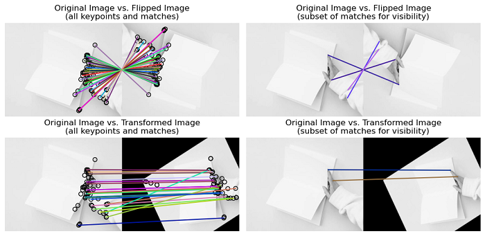
Example

The following example applies transformations (rotation and affine transformation), to the input image and detects keypoints and extracts descriptors using the SIFT algorithm.

import matplotlib.pyplot as plt
from skimage import io, transform, color, feature, io

# Load the input image and apply transformations
image = color.rgb2gray(io.imread('Images/book.jpg'))
flipped_image = transform.rotate(image, 180)
affine_transform = transform.AffineTransform(scale=(1.3, 1.1), rotation=0.5, translation=(0, -200))
transformed_image = transform.warp(image, affine_transform)

# Initialize the SIFT descriptor extractor
descriptor_extractor = feature.SIFT()

# Detect and extract keypoints and descriptors for each image
def detect_and_extract_features(image):
   descriptor_extractor.detect_and_extract(image)
   keypoints = descriptor_extractor.keypoints
   descriptors = descriptor_extractor.descriptors
   return keypoints, descriptors

# Detect keypoints and extract descriptors for the original image
keypoints1, descriptors1 = detect_and_extract_features(image)

# Detect keypoints and extract descriptors for the flipped image
keypoints2, descriptors2 = detect_and_extract_features(flipped_image)

# Detect keypoints and extract descriptors for the transformed image
keypoints3, descriptors3 = detect_and_extract_features(transformed_image)

# Match descriptors between images
matches12 = feature.match_descriptors(descriptors1, descriptors2, max_ratio=0.6, cross_check=True)
matches13 = feature.match_descriptors(descriptors1, descriptors3, max_ratio=0.6, cross_check=True)

# Create subplots for displaying images and matches
fig, ax = plt.subplots(nrows=2, ncols=2, figsize=(10, 5))
plt.gray()

# Plot matches between original and flipped images
feature.plot_matches(ax[0, 0], image, flipped_image, keypoints1, keypoints2, matches12)
ax[0, 0].axis('off')
ax[0, 0].set_title("Original Image vs. Flipped Image&bsol;n(all keypoints and matches)")

# Plot matches between original and transformed images
feature.plot_matches(ax[1, 0], image, transformed_image, keypoints1, keypoints3, matches13)
ax[1, 0].axis('off')
ax[1, 0].set_title("Original Image vs. Transformed Image&bsol;n(all keypoints and matches)")

# Plot a subset of matches for visibility between original and flipped images
feature.plot_matches(ax[0, 1], image, flipped_image, keypoints1, keypoints2, matches12[::15], only_matches=True)
ax[0, 1].axis('off')
ax[0, 1].set_title("Original Image vs. Flipped Image&bsol;n(subset of matches for visibility)")

# Plot a subset of matches for visibility between original and transformed images
feature.plot_matches(ax[1, 1], image, transformed_image, keypoints1, keypoints3, matches13[::15], only_matches=True)
ax[1, 1].axis('off')
ax[1, 1].set_title("Original Image vs. Transformed Image&bsol;n(subset of matches for visibility)")

plt.tight_layout()
plt.show()

Output

Print Page