Scikit Image - Shape Index

The shape index is indeed a single-valued measure of local curvature, and it's derived from the eigenvalues of the Hessian matrix, defined by Koenderink & van Doorn. It can be used to characterize and classify local structures in an image based on their apparent local shape. The shape index values map to a range from -1 to 1, allowing for the identification and differentiation of various shapes within an image.

The specific ranges of the shape index and their corresponding shapes are as follows −

[-1, -7/8): Spherical cup
[-7/8, -5/8): Through
[-5/8, -3/8): Rut
[-3/8, -1/8): Saddle rut
[-1/8, +1/8): Saddle
[+1/8, +3/8): Saddle ridge
[+3/8, +5/8): Ridge
[+5/8, +7/8): Dome
[+7/8, +1]: Spherical cap

These different types of shapes, make it a valuable tool for shape analysis and pattern recognition in image processing and computer vision applications. By examining the shape index values at different points in an image, it can be easy to classify and extract information about the local shapes, which can be particularly useful in tasks such as object recognition and segmentation.

Using the skimage.feature.shape_index() function

The skimage library provides the shape_index() function within its feature module to compute the shape index of an input image. The shape index is a measure of local curvature in the image defined by Koenderink and van Doorn, assuming that the image represents a 3D plane with pixel intensities representing heights.

It is derived from the eigenvalues of the Hessian, and its values range from -1 to 1. In flat regions of the image, the shape index is undefined and is represented as NaN.

Syntax

Here is the syntax of the function −

skimage.feature.shape_index(image, sigma=1, mode='constant', cval=0)

Parameters

The details of the parameters are explained below −

image (M, N) ndarray: This is the input image on which the shape index will be computed.
sigma (float, optional): This specifies the standard deviation used for the Gaussian kernel, which is applied to the input image to smooth it before calculating the Hessian eigen values.
mode (str, optional): This parameter determines how to handle values outside the image borders. The options are 'constant', 'reflect', 'wrap', 'nearest', 'mirror'.
cval (float, optional): This is used in conjunction with the 'constant' mode. It specifies the value to use for filling in regions outside the image boundaries when mode is set to 'constant'.

The function returns a ndarray (s) that is the computed shape index.

Example

This example demonstrates how to use the shape_index function to analyze the local curvature or shape characteristics of a specific region within an image.

import numpy as np
from skimage.feature import shape_index

# Create a 5x5 image with a square-shaped region
square = np.zeros((5, 5))
square[2, 2] = 4 

# Display the input 
print('Input Square:')
print(square)

# Compute the shape index with a specified sigma value
s = shape_index(square, sigma=0.1)

# Display the computed shape index values
print("Shape Index:")
print(s)

Output

Input Square:
[[0. 0. 0. 0. 0.]
 [0. 0. 0. 0. 0.]
 [0. 0. 4. 0. 0.]
 [0. 0. 0. 0. 0.]
 [0. 0. 0. 0. 0.]]

Shape Index:
[[ nan  nan -0.5  nan  nan]
 [ nan -0.   nan -0.   nan]
 [-0.5  nan -1.   nan -0.5]
 [ nan -0.   nan -0.   nan]
 [ nan  nan -0.5  nan  nan]]

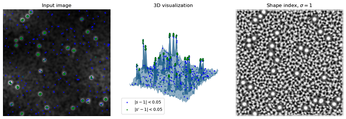
Example

The following example generates a test image with random noise, uneven illumination, and spots, and then computes the shape index of that image using the shape_index() function.

import numpy as np
import matplotlib.pyplot as plt
from scipy import ndimage as ndi
from skimage.feature import shape_index
from skimage.draw import disk

# Function to create a test image with random noise, spots, and uneven illumination
def create_test_image(image_size=256, spot_count=30, spot_radius=5, cloud_noise_size=4):
   rng = np.random.default_rng()
   image = rng.normal(loc=0.25, scale=0.25, size=(image_size, image_size))
   
   for _ in range(spot_count):
      rr, cc = disk(
         (rng.integers(image.shape[0]), rng.integers(image.shape[1])),
         spot_radius,
         shape=image.shape
      )
      image[rr, cc] = 1
   
   image *= rng.normal(loc=1.0, scale=0.1, size=image.shape)
   
   image *= ndi.zoom(
      rng.normal(loc=1.0, scale=0.5, size=(cloud_noise_size, cloud_noise_size)),
      image_size / cloud_noise_size
   )
   
   return ndi.gaussian_filter(image, sigma=2.0)

# Create the test image and compute its shape index
image = create_test_image()
s = shape_index(image)

# Define the target shape (spherical cap) and a threshold delta
target = 1
delta = 0.05

# Find points in the shape index map that are close to the target shape
point_y, point_x = np.where(np.abs(s - target) < delta)
point_z = image[point_y, point_x]

# Apply Gaussian smoothing to the shape index map to reduce noise
s_smooth = ndi.gaussian_filter(s, sigma=0.5)

# Find smoothed points close to the target shape
point_y_s, point_x_s = np.where(np.abs(s_smooth - target) < delta)
point_z_s = image[point_y_s, point_x_s]

# Create a figure to display the results
fig = plt.figure(figsize=(12, 4))

# Plot the input image
ax1 = fig.add_subplot(1, 3, 1)
ax1.imshow(image, cmap=plt.cm.gray)
ax1.axis('off')
ax1.set_title('Input image')

# Scatter plot of points representing the detected shapes
scatter_settings = dict(alpha=0.75, s=10, linewidths=0)
ax1.scatter(point_x, point_y, color='blue', **scatter_settings)
ax1.scatter(point_x_s, point_y_s, color='green', **scatter_settings)

# 3D visualization of the image with points representing shapes
ax2 = fig.add_subplot(1, 3, 2, projection='3d', sharex=ax1, sharey=ax1)
x, y = np.meshgrid(
   np.arange(0, image.shape[0], 1),
   np.arange(0, image.shape[1], 1)
)
ax2.plot_surface(x, y, image, linewidth=0, alpha=0.5)
ax2.scatter(point_x, point_y, point_z, color='blue', label='$|s - 1|<0.05$', **scatter_settings)
ax2.scatter(point_x_s, point_y_s, point_z_s, color='green', label='$|s&bsol;' - 1|<0.05$', **scatter_settings)
ax2.legend(loc='lower left')
ax2.axis('off')
ax2.set_title('3D visualization')

# Plot the shape index map
ax3 = fig.add_subplot(1, 3, 3, sharex=ax1, sharey=ax1)
ax3.imshow(s, cmap=plt.cm.gray)
ax3.axis('off')
ax3.set_title(r'Shape index, $&bsol;sigma=1$')

fig.tight_layout()
plt.show()

Output

Print Page